Fitting with highly configurable multi layer perceptrons
The fitting of functions, curves and surfaces with a neural network is a classic machine learning problem and it does not require any sophisticated neural network architecture in order to get a fitting with accuracy close to 100%:
it is enough an MLP (Multi-Layer Perceptron) where both the input and output layers contain only one neuron because the dimension of both domain and codomain is 1
and some freedom of choice in hidden layer architecture, their own activation functions, loss function, optimizator and several training parameters.
On Internet you can find several examples of MLPs that fit this kind of functions; however often such examples combine in a single Python script dataset generation (and function to fit usually hardcoded), MLP training,
prediction and result visualization; also the architecture of the neural network is hardcoded and/or is not very parameterizable via command line and finally the activation functions, the used optimizer and the loss function are decided by the author
without any explanation describing the reasons for their choice.
Poor parameterization, the use of hard-coded implemented choices and unification of various functionalities in a single script make experimentation difficult
and they force the experimenter to proceed for code changes in order to implement and test MLP customizations and/or training procedures.
Goal of this series of posts on the fitting of functions, curves and surfaces is to allow the user to experience different combinations of MLP architectures, their own activation functions, training algorithm and loss function without writing code but working only on the command line of the four Python scripts which separately implement the following features:
- Dataset generation: generation of a csv file from a mathematical object passed as argument (therefore not hardcoded). This phase not mandatory, in fact datasets could be pre-existing (as it happens in the real world, for example by extracting curves from data present in databases or Excel files, from the output of measuring instruments, from data-loggers connected to electronic sensors, etc) and therefore not necessarily be generated in a synthetic way.
- MLP architecture definition + Training: configuration of MLP hidden layer architecture with their own activation functions and training procedure execution on training dataset allowing you to specify your choice of optimization algorithm, loss function and other training parameters.
- Prediction: application of the previously trained model to an input dataset (which should contain data never seen by the model being trained) and generation of an output csv file containing the prediction.
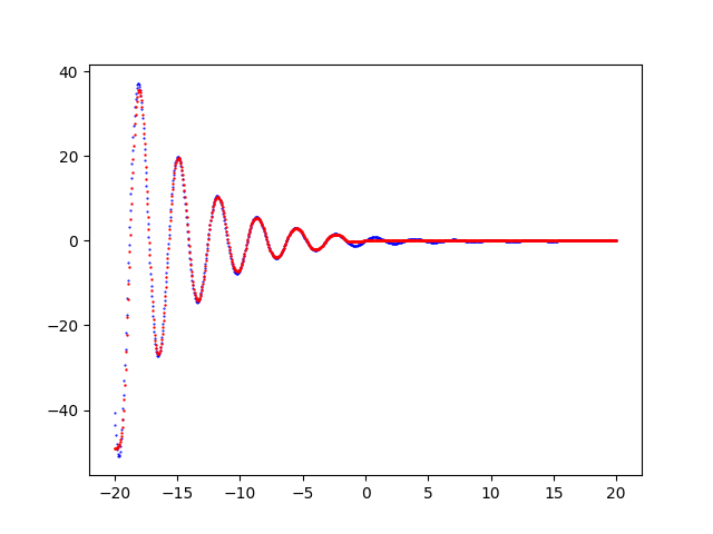
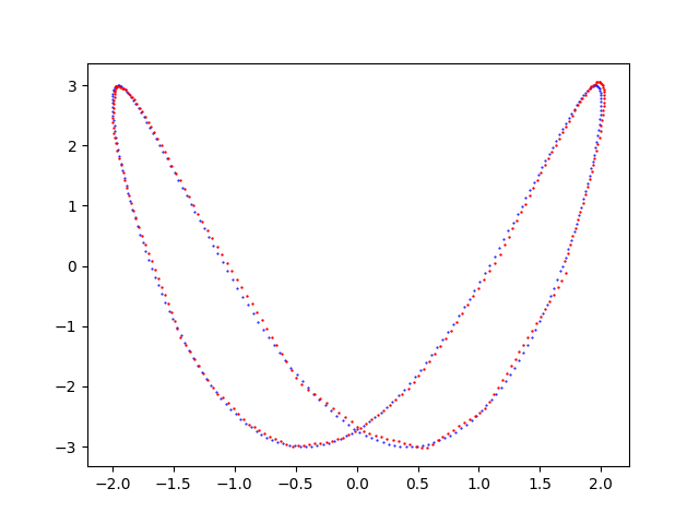
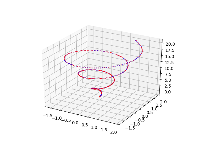
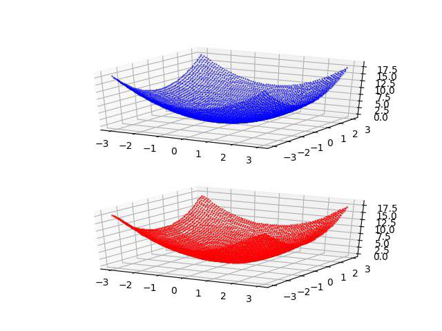
- Visualization of the result: generation of a chart that shows overlapped the initial dataset curve (training or test, as you prefer) and prediction curve and it allows the visual comparison of the two curves. This phase is not mandatory because the prediction is saved in the previous step in a csv file and therefore it is already usable as such.
Links to posts and code
The following table allows you to access the specific posts and the relative code of the various types of fitters: please click on icon to show the correspondent post and on icon to get the code available on GitHub.