One-variable real-valued function fitting with TensorFlow
This post is part of a series of posts on the fitting of mathematical objects (functions, curves and surfaces) through a MLP (Multi-Layer Perceptron) neural network;
for an introduction on the subject please see the post Fitting with highly configurable multi layer perceptrons.
The topic of this post is the fitting of a continuous and limited real-valued function defined in a closed interval of the reals $$f(x) \colon [a,b] \to \rm I\!R$$ with a MLP
so that the user can test different combinations of MLP architectures, their own activation functions, training algorithm and loss function without writing code
but working only on the command line of the six Python scripts which implement the following features:
- Dataset generation
- MLP architecture definition + Training
- Prediction
- Visualization of the result
- Diagnostics
To get the code please see the paragraph Download of the complete code at the end of this post.
The exact same mechanism was created using PyTorch technology; see the post One-variable real-valued function fitting with PyTorch always published on this website.
Dataset generation
Goal of the fx_gen.py Python program
is to generate datasets (both training and test ones) to be used in later phases;
it takes in command line the function to be approximated (in lambda body syntax), the interval of independent variable (begin, end and discretization step)
and it generates the dataset in an output csv file applying the function to the passed interval.
In fact the output csv file has two columns (with header): first column contains the sorted values of independent variable $x$ within the passed interval discretized by discretization step;
second column contains the values of dependent variable, ie the values of function $f(x)$ correspondent to values of $x$ of first column.
To get the program usage you can run this following command:
$ python fx_gen.py --helpusage: fx_gen.py [-h]
-h, --help show this help message and exit
--dsout DS_OUTPUT_FILENAME dataset output file (csv format)
--fx FUNC_X_BODY f(x) body (body lamba format)
--rbegin RANGE_BEGIN begin range (default:-5.0)
--rend RANGE_END end range (default:+5.0)
--rstep RANGE_STEP step range (default: 0.01)An example of using the program fx_gen.py
Suppose you want to approximate the function $$f(x)=\frac{\sin 2x}{e^\frac{x}{5}}$$ in the range $[-20.0,20.0]$. Keeping in mind that np is the alias of NumPy library, the translation of this function in lambda body Python syntax is:
np.sin(2 * x) / np.exp(x / 5)$ python fx_gen.py \
--dsout mytrain.csv \
--fx "np.sin(2 * x) / np.exp(x / 5)" \
--rbegin -20.0 \
--rend 20.0 \
--rstep 0.01$ python fx_gen.py \
--dsout mytest.csv \
--fx "np.sin(2 * x) / np.exp(x / 5)" \
--rbegin -20.0 \
--rend 20.0 \
--rstep 0.0475MLP architecture definition + Training
Goal of the fx_fit.py Python program
is to dynamically create a MLP and perform its training according to the passed parameters through the command line.
To get the program usage you can run this following command:
$ python fx_fit.py --helpusage: fx_fit.py [-h]
--trainds TRAIN_DATASET_FILENAME
--modelout MODEL_PATH
[--valds VAL_DATASET_FILENAME]
[--bestmodelmonitor BEST_MODEL_MONITOR]
[--epochs EPOCHS]
[--batch_size BATCH_SIZE]
[--hlayers HIDDEN_LAYERS_LAYOUT [HIDDEN_LAYERS_LAYOUT ...]]
[--hactivations ACTIVATION_FUNCTIONS [ACTIVATION_FUNCTIONS ...]]
[--winitializers KERNEL_INITIALIZERS [KERNEL_INITIALIZERS ...]]
[--binitializers BIAS_INITIALIZERS [BIAS_INITIALIZERS ...]]
[--optimizer OPTIMIZER]
[--loss LOSS]
[--metrics METRICS [METRICS ...]]
[--dumpout DUMPOUT_PATH]
[--logsout LOGSOUT_PATH]
[--modelsnapout MODEL_SNAPSHOTS_PATH]
[--modelsnapfreq MODEL_SNAPSHOTS_FREQ]An example of using the program fx_fit.py
Suppose you have a training dataset available (for example generated through fx_gen.py program as shown in the previous paragraph)
and you want the MLP to have three hidden layers with respectively with 200, 300 and 200 neurons and that you want to use the sigmoid activation function output from all three layers;
moreover you want to perform 1000 training epochs with a 200 items batch size using the Adamax optimizator algorithm with learning rate equal to 0.02
and loss function equal to MeanSquaredError. To put all this into action, run the following command:
$ python fx_fit.py \
  --trainds mytrain.csv \
  --modelout mymodel \
  --hlayers 200 300 200 \
  --hactivation sigmoid sigmoid sigmoid \
  --epochs 1000 \
  --batch_size 200 \
  --optimizer 'Adamax(learning_rate=0.02)' \
--loss 'MeanSquaredError()'mymodel will contain the MLP model trained on mytrain.csv dataset according to the parameters passed on the command line.
Prediction
Goal of the fx_predict.py Python program
is to apply the MLP model generated through fx_fit.py to an input dataset (for example the test dataset generated through fx_gen.py program as shown in a previous paragraph);
the execution of the program produces in output a csv file with two columns (with header): the first column contains the values of indepedent variable $x$ taken from test dataset
and the second column contains the predicted values of dependent variable, ie the values of the prediction correspondent to values of $x$ of first column.
To get the program usage you can run this following command:
$ python fx_predict.py --helpusage: fx_predict.py [-h]
--model MODEL_PATH
--ds DATASET_FILENAME
--predictionout PREDICTION_DATA_FILENAMEAn example of using the program fx_predict.py
Suppose you have the test dataset mytest.csv available (for example generated through fx_gen.py program as shown in a previous paragraph)
and the trained model of MLP in the folder mymodel (generated through fx_fit.py program as shown in the example of previous paragraph); run the following command:
$ python fx_predict.py \
  --model mymodel \
  --ds mytest.csv \
  --predictionout myprediction.csv
myprediction.csv will contain the fitting of the initial function.
Visualization of the result
Goal of the fx_scatter.py Python program
is to visualize the prediction curve superimposed on initial dataset curve (test or training, as you prefer) and it allows the visual comparison of the two curves.
To get the program usage you can run this following command:
$ python fx_scatter.py --helpusage: fx_scatter.py [-h]
--ds DATASET_FILENAME
--prediction PREDICTION_DATA_FILENAME
[--title FIGURE_TITLE]
[--savefig SAVE_FIGURE_FILENAME]An example of using the program fx_scatter.py
Having the test dataset mytest.csv available (for example generated through fx_gen.py program as shown in a previous paragraph)
and the prediction csv file (generated through fx_predict.py program as shown in the previous paragraph), to generate the two xy-scatter charts, execute the following command:
$ python fx_scatter.py \
  --ds mytest.csv \
--prediction myprediction.csvNote: Given the stochastic nature of the training phase, your specific results may vary. Consider running the example a few times.
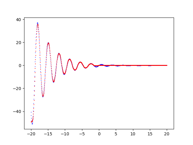
Chart generated by the program
fx_scatter.py that shows the fitting of the function $f(x)=\frac{\sin 2x}{e^\frac{x}{5}}$ made by the MLP.Diagnostics
The diagnostics consists of a series of techniques to analyze the behavior of MLP during the training phase,
so that the program fx_fit.py supports the following command line arguments in order to export information so that other programs can then analyze it:
[--metrics METRICS [METRICS ...]]
[--dumpout DUMPOUT_PATH]
[--logsout LOGSOUT_PATH]
[--modelsnapout MODEL_SNAPSHOTS_PATH]
[--modelsnapfreq MODEL_SNAPSHOTS_FREQ]
--metrics is the list of metrics to be calculated on the training dataset and, if specified by argument --valds, also on the validation dataset.--dumpout is the argument to indicate the directory where to save the values of the loss function and the calculated metrics in csv format.--logsout is the argument to indicate the directory where to save the log files to allow TensorBoard to analyze them (both during the training phase and at the end of training).--modelsnapout is the argument to indicate the directory where to save the model of each --modelsnapfreq epochs; the first and last epochs are always saved if this argument is specified.--modelsnapfreq indicates how many times to save the model in the directory indicated by --modelsnapout.
The value of the calculated metrics and the value of the loss function is available on the output stream of fx_fit.py.
The information exported from fx_fit.py can be used by the following 3 programs:
- TensorBoard
- fx_diag.py
- fx_video.py
$ tensorboard --logdir path/to/logdir--logdir is the same directory generated by fx_fit.py specified by argument--logsout.See TensorBoard for details.
The Python program
fx_diag.py
generate a series of graphs showing the curve of the loss function and the curves of the metrics calculated on the training dataset
and also on the validation dataset if this has been passed to fx_fit.py with the option --valds.To get the program usage you can run this following command:
$ python fx_diag.py --helpusage: fx_diag.py [-h] [--help]
--dump DUMP_PATH
[--savefigdir SAVE_FIGURE_DIRECTORY]The Python program
fx_video.py
generates an animated git that shows the prediction curve computed on an input dataset as the epochs change.To get the program usage you can run this following command:
$ python fx_video.py --helpusage: fx_videp.py [-h] [--help]
--modelsnap MODEL_SNAPSHOTS_PATH
--ds DATASET_FILENAME
--savevideo SAVE_GIF_VIDEO
[--fps FPS]
[--width WIDTH]
[--height HEIGHT]--modelsnap is the directory generated by fx_fit-py and specified via the parameter --modelsnapout.Please read the file README.md for a complete detail of the semantics of the parameters supported on the command line.
Examples of cascade use of these programs
In the folder one-variable-function-fitting/examples
there are nine shell scripts that show the use in cascade of these programs in various combinations of parameters
(MLP architecture, activation functions, optimization algorithm, loss function, metrics, best model, initializers, training procedure parameters, diagnostics)
To run the nine examples, run the following commands:
$ cd one-variable-function-fitting/examples
$ sh example1.sh
$ sh example2.sh
$ sh example3.sh
$ sh example4.sh
$ sh example5.sh
$ sh example6.sh
$ sh example7.sh
$ sh example8.sh
$ sh example9.shMedia
Download of the complete code
The complete code is available at GitHub.
These materials are distributed under MIT license; feel free to use, share, fork and adapt these materials as you see fit.
Also please feel free to submit pull-requests and bug-reports to this GitHub repository or contact me on my social media channels available on the top right corner of this page.