Solving delay differential equations using numerical methods in Python
The delay differential equations are used in the mathematical modeling of systems where the reactions to the stresses
occur not immediately but after a certain non-negligible period of time.
Delay Differential equations are a wide and complicated field of mathematics still under research;
the analytical resolution of such equations is, when feasible, certainly not trivial: see the post on this site A method to solve first-order time delay differential equation using Lambert W function
for a discussion of the analytical solution of a particular class of such equations.
This post instead deals with numerical solving techniques in Python using two different libraries: ddeint
and jitcdde;
ddeint is based on Scipy while jitcdde produces C code that is compiled and executed.
This post does not go into the implementation of these two libraries, but focuses on usage, proceeding by examples
with increasing complexity.
All of the various code examples described in this post require Python version 3 and the NumPy and MatPlotLib libraries;
additionally, ddeint based scripts require SciPy for the above, while jitcdde based scripts require SymPy.
To get the code see the Full code download paragraph at the bottom of this post.
Conventions
In this post the conventions used are as follows:
- DDE stands for Delay Differential Equation.
- ODE stands for Ordinary Differential Equation.
- IVP stands for Initial Value Problem, also called Cauchy problem.
- $t$ is the independent variable, it indicates the time and is expressed in seconds.
- $y$ is the unknown function and is intended as a function of t, i.e. $y=y(t)$, but the use of this compact notation, in addition to having a greater readability at a mathematical level makes it easier to "translate" the equation into code.
- $y_1$ and $y_2$ are the unknown functions in the case of systems of two equations.
- The instant $t=0$ is assumed as initial time, so in the following examples it will always be $t_0=0$.
-
$\phi$ stands for the initial historical function, i.e., the function that gives the values of the unknown function $y$
for values of $t \leq t_0$.
-
$\tau$ denotes the delay function, it is intended as a function of $t$ and $y$, i.e. $\tau=f(t, y(t))$.
- $y'$ is the first derivative of $x$ with respect to $t$.
- $y''$ is the second derivative of $x$ with respect to $t$.
Observations on the initial conditions of DDEs
In the case of an ODE in an IVP in addition to the equation are given many initial conditions depending on the order of the equation
and are of the form: $y(t_0)=y_0$, $y'(t_0)=y'_0$, and so on
(for a complete list of other conditions to guarantee the existence and uniqueness of the solution see the Picard-Lindelöf theorem).
For DDEs, on the other hand, it is not enough to give a set of initial values for the function and its derivatives at $t_0$, but one must give a set of functions to provide
the historical values for $t_0 - max(\tau) \leq t \leq t_0$.
How many and which historical functions to give to get a unique solution depends on the order of the equation: for a first-order equation you only need to give one $\phi$ to give the historical values of $y$.
For a second-order equation we must give an $\phi$ to give the historical values of $y$ and another $\phi$ to give the historical values of $y'$.
For a system of first-order equations, one must give two $\phi$ to provide the historical values of $y_1$ and $y_2$. And so on.
Technical notes
While, as mentioned above, this post does not go into detail about the implementation, it is important to provide a few technical notes
before proceeding with the examples.
ddeint
ddeint is a Python library that contains a class of the same name, which is the heart of the implementation, whose purpose is to override some functions of scipy.integrate.ode to allow the update of a pseudo-variable (representing the unknown function) at each integration step; the library has been developed by Zulko, the source is available at the address https://github.com/Zulko/ddeint and the library is installable with the following command:
$ pip install ddeintSyntactical notes
In the code, the definition of the DDE (or DDE system) is a Python function with at least two arguments:
- the first argument is the unknown (usually named
Y); - the second argument is time (usually named
t).
Y, i.e., the unknown, is a tuple that contains a slot for each component of the unknown:
so for a single first-order DDE, the tuple Y has only one slot, while in a system with two unknowns $y_1$ and $y_2$,
the tuple Y has two slots, and so on.The function that defines the DDE (or system of DDEs) may have additional arguments that are used to implement a parametric DDE (or parametric systems of DDEs); Example #6 shows the resolution of a parametric system of two DDEs.
The name of the Python function that defines the equation is free: in the following examples will be
equation; often, on the Internet, it is model.Here is an example of a DDE (so only one unknown, so
Y is a tuple of one slot) that is not parametric:
def equation(Y, t):
return -Y(t - 1)d is the parameter) of two DDEs (so Y has two slots):
def equation(Y, t, d):
    x,y = Y(t)
    xd,yd = Y(t-d)
    return [x * yd, y * xd]
JiTCDDE
JiTCDDE stands for just-in-time compilation of DDEs; it takes an iterable of SymPy expressions, translates them into C code, compiles them on the fly and invokes the compiled code from Python; the library has been developed by Neurophysik, the source is available at the address https://github.com/neurophysik/jitcddet and the library is installable with the following command:
$ pip install jitcddeSyntactical notes
In the code, the definition of the DDE (or system of DDEs) is a Python list; for each element in the list, these rules apply:
-
the name
yis the unknown; it is a SymPy symbolic name imported fromjitcdde; y in turn is a Python function where the first argument is the component index of the unknown itself while the second argument is the timet; - the name
tis the time; this is also a SymPy symbolic name imported fromjitcdde
Additional SymPy symbols can be used in the list defining the DDE (or DDE system), which must be explicitly instantiated with
symengine.symbols and they are used to implement parametric DDEs (or parametric systems of DDEs);
example #6 shows the resolution of a parametric system of two DDEs.The name of the variable that contains the list of equations is free: in the following examples will be
equation or equations; often, on the Internet, it is f.Here is an example of a DDE (so only one unknown, so
y can have the value 0 as the first argument) that is not parametric:
equation = [-y(0, t-1.)]d is the parameter) of two DDEs (so y can have the value 0 and 1 as the first argument):
d=symengine.symbols("d")
equations=[
	y(0, t) * y(1, t-d),
	y(1, t) * y(0, t-d)]
Example #1: First-order DDE with one constant delay and a constant initial history function
Let the following DDE be given: $$ y'(t)=-y(t-1) $$ where the delay is $1 s$; the example compares the solutions of three different cases using three different constant history functions:
- Case #1: $\phi(t)=-1$
- Case #2: $\phi(t)=0$
- Cas3 #3: $\phi(t)=1$
ddeint
Below is an example of Python code that numerically solves the DDE using ddeint:
import numpy as np
import matplotlib.pyplot as plt
from ddeint import ddeint

def equation(Y, t):
    return -Y(t - 1)

def initial_history_func_m1(t):
    return -1.

def initial_history_func_0(t):
    return 0.

def initial_history_func_p1(t):
    return 1.

plt.rcParams['font.size'] = 8
fig, axs = plt.subplots(3, 1)
fig.tight_layout(rect=[0, 0, 1, 0.95], pad=3.0)
fig.suptitle("$y'(t)=-y(t-1)$ solved by ddeint")

ts = np.linspace(0, 20, 2000)

ys = ddeint(equation, initial_history_func_m1, ts)
axs[0].plot(ts, ys, color='red', linewidth=1)
axs[0].set_title('$ihf(t)=-1$')

ys = ddeint(equation, initial_history_func_0, ts)
axs[1].plot(ts, ys, color='red', linewidth=1)
axs[1].set_title('$ihf(t)=0$')

ys = ddeint(equation, initial_history_func_p1, ts)
axs[2].plot(ts, ys, color='red', linewidth=1)
axs[2].set_title('$ihf(t)=1$')

plt.show()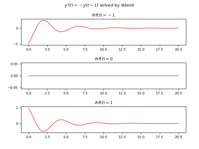
Graph of the numerical solutions of the DDE in the three cases obtained by ddeint.
JiTCDDE
Below is an example of Python code that numerically solves the DDE using JiTCDDE:
import numpy as np
import matplotlib.pyplot as plt
from jitcdde import jitcdde, y, t

equation = [-y(0, t-1.)]
dde = jitcdde(equation)

plt.rcParams['font.size'] = 8
fig, axs = plt.subplots(3, 1)
fig.tight_layout(rect=[0, 0, 1, 0.95], pad=3.0)
fig.suptitle("$y'(t)=-y(t-1)$ solved by jitcdde")

ts = np.linspace(0, 20, 2000)

dde.constant_past([-1.])
ys = []
for t in ts:
	ys.append(dde.integrate(t))
axs[0].plot(ts, ys, color='red', linewidth=1)
axs[0].set_title('$ihf(t)=-1$')

dde.constant_past([0])
ys = []
for t in ts:
	ys.append(dde.integrate(t))
axs[1].plot(ts, ys, color='red', linewidth=1)
axs[1].set_title('$ihf(t)=0$')

dde.constant_past([1.])
ys = []
for t in ts:
	ys.append(dde.integrate(t))
axs[2].plot(ts, ys, color='red', linewidth=1)
axs[2].set_title('$ihf(t)=1$')

plt.show()
Graph of the numerical solutions of the DDE in the three cases obtained by JiTCDDE.
Example #2: First-order DDE with one constant delay and a non constant initial history function
Let the following DDE be given: $$ y'(t)=-y(t-2) $$ where the delay is $2 s$; the example compares the solutions of four different cases using two different non constant history functions and two different intervals of $t$:
- Case #1: $\phi(t)=e^{-t} - 1, t \in [0, 4]$
- Case #2: $\phi(t)=e^{t} - 1, t \in [0, 4]$
- Case #3: $\phi(t)=e^{-t} - 1, t \in [0, 60]$
- Case #4: $\phi(t)=e^{t} - 1, t \in [0, 60]$
ddeint
Below is an example of Python code that numerically solves the DDE using ddeint:
import numpy as np
import matplotlib.pyplot as plt
from ddeint import ddeint

def equation(Y, t):
    return -Y(t - 2)

def initial_history_func_exp_mt(t):
    return np.exp(-t) - 1

def initial_history_func_exp_pt(t):
    return np.exp(t) - 1

plt.rcParams['font.size'] = 8
fig, axs = plt.subplots(2, 2)
fig.tight_layout(rect=[0, 0, 1, 0.95], pad=3.0)
fig.suptitle("$y'(t)=-y(t-2)$ solved by ddeint")

ts = np.linspace(0, 4, 2000)

ys = ddeint(equation, initial_history_func_exp_mt, ts)
axs[0, 0].plot(ts, ys, color='red', linewidth=1)
axs[0, 0].set_title('$ihf(t)=e^-t - 1, t \in [0, 4]$')

ys = ddeint(equation, initial_history_func_exp_pt, ts)
axs[0, 1].plot(ts, ys, color='red', linewidth=1)
axs[0, 1].set_title('$ihf(t)=e^t - 1, t \in [0, 4]$')

ts = np.linspace(0, 60, 2000)

ys = ddeint(equation, initial_history_func_exp_mt, ts)
axs[1, 0].plot(ts, ys, color='red', linewidth=1)
axs[1, 0].set_title('$ihf(t)=e^-t - 1, t \in [0, 60]$')

ys = ddeint(equation, initial_history_func_exp_pt, ts)
axs[1, 1].plot(ts, ys, color='red', linewidth=1)
axs[1, 1].set_title('$ihf(t)=e^t - 1, t \in [0, 60]$')

plt.show()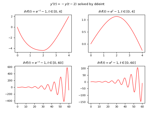
Graph of the numerical solutions of the DDE in the four cases obtained by ddeint.
JiTCDDE
Below is an example of Python code that numerically solves the DDE using JiTCDDE:
import numpy as np
import matplotlib.pyplot as plt
from jitcdde import jitcdde, y, t

equation= [-y(0, t-2.)]
dde = jitcdde(equation)

def initial_history_func_exp_mt(t):
    return [np.exp(-t) - 1]

def initial_history_func_exp_pt(t):
    return [np.exp(t) - 1]

plt.rcParams['font.size'] = 8
fig, axs = plt.subplots(2, 2)
fig.tight_layout(rect=[0, 0, 1, 0.95], pad=3.0)
fig.suptitle("$y'(t)=-y(t-2)$ solved by jitcdde")

ts = np.linspace(0, 4, 2000)

dde.past_from_function(initial_history_func_exp_mt)
ys = []
for t in ts:
	ys.append(dde.integrate(t))
axs[0, 0].plot(ts, ys, color='red', linewidth=1)
axs[0, 0].set_title('$ihf(t)=e^-t - 1, t \in [0, 4]$')

dde.past_from_function(initial_history_func_exp_pt)
ys = []
for t in ts:
	ys.append(dde.integrate(t))
axs[0, 1].plot(ts, ys, color='red', linewidth=1)
axs[0, 1].set_title('$ihf(t)=e^t - 1, t \in [0, 4]$')

ts = np.linspace(0, 60, 2000)

dde.past_from_function(initial_history_func_exp_mt)
ys = []
for t in ts:
	ys.append(dde.integrate(t))
axs[1, 0].plot(ts, ys, color='red', linewidth=1)
axs[1, 0].set_title('$ihf(t)=e^-t - 1, t \in [0, 60]$')

dde.past_from_function(initial_history_func_exp_mt)
ys = []
for t in ts:
	ys.append(dde.integrate(t))
axs[1, 1].plot(ts, ys, color='red', linewidth=1)
axs[1, 1].set_title('$ihf(t)=e^t - 1, t \in [0, 60]$')

plt.show()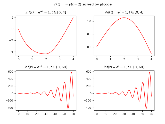
Graph of the numerical solutions of the DDE in the four cases obtained by JiTCDDE.
Example #3: First-order DDE with one non constant delay and a constant initial history function
Let the following DDE be given: $$ y'(t)=y(t-delay(y, t))$$ where the delay is not constant and is given by the function $delay(y, t)=|\frac{1}{10} t y(\frac{1}{10} t)|$; the example compares the solutions of two different cases using two different constant history functions:
- Case #1: $\phi(t)=-1$
- Case #2: $\phi(t)=1$
ddeint
Below is an example of Python code that numerically solves the DDE using ddeint:
import numpy as np
import matplotlib.pyplot as plt
from ddeint import ddeint

def delay(Y, t):
    return np.abs(0.1 * t * Y(0.1 * t))

def equation(Y, t):
    return Y(t - delay(Y, t))

def initial_history_func_m1(t):
    return -1.

def initial_history_func_p1(t):
    return 1.

plt.rcParams['font.size'] = 8
fig, axs = plt.subplots(2, 1)
fig.tight_layout(rect=[0, 0, 1, 0.95], pad=3.0)
fig.suptitle("$y'(t)=y(t-delay(y, t))$ solved by ddeint")

ts = np.linspace(0, 50, 10000)

ys = ddeint(equation, initial_history_func_m1, ts)
axs[0].plot(ts, ys, color='red', linewidth=1)
axs[0].set_title('$ihf(t)=-1$')

ys = ddeint(equation, initial_history_func_p1, ts)
axs[1].plot(ts, ys, color='red', linewidth=1)
axs[1].set_title('$ihf(t)=1$')

plt.show()Graph of the numerical solutions of the DDE in the two cases obtained by ddeint.
JiTCDDE
Below is an example of Python code that numerically solves the DDE using JiTCDDE:
import numpy as np
import matplotlib.pyplot as plt
from jitcdde import jitcdde, y, t

def delay(y, t):
    return np.abs(0.1 * t * y(0, 0.1 * t))

equation = [y(0, t - delay(y, t))]
dde = jitcdde(equation, max_delay=1000)

plt.rcParams['font.size'] = 8
fig, axs = plt.subplots(2, 1)
fig.tight_layout(rect=[0, 0, 1, 0.95], pad=3.0)
fig.suptitle("$y'(t)=y(t-delay(y, t))$ solved by jitcdde")

ts = np.linspace(0, 50, 10000)

dde.constant_past([-1.])
ys = []
for t in ts:
	ys.append(dde.integrate(t))
axs[0].plot(ts, ys, color='red', linewidth=1)
axs[0].set_title('$ihf(t)=-1$')

dde.constant_past([1.])
ys = []
for t in ts:
	ys.append(dde.integrate(t))
axs[1].plot(ts, ys, color='red', linewidth=1)
axs[1].set_title('$ihf(t)=1$')

plt.show()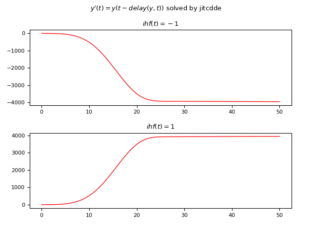
Graph of the numerical solutions of the DDE in the two cases obtained by JiTCDDE.
Example #4: First-order DDE with one non constant delay and a non constant initial history function
Let the following DDE be given: $$ y'(t)=y(t-delay(y, t))$$ where the delay is not constant and is given by the function $delay(y, t)=|\frac{1}{10} t y(\frac{1}{10} t)|$ and the initial historical function is non-constant and is $\phi(t)=e^t$.
ddeint
Below is an example of Python code that numerically solves the DDE using ddeint:
import numpy as np
import matplotlib.pyplot as plt
from ddeint import ddeint

def delay(Y, t):
    return np.abs(0.1 * t * Y(0.1 * t))

def equation(Y, t):
    return Y(t - delay(Y, t))

def initial_history_func_exp_pt(t):
    return np.exp(t)

plt.rcParams['font.size'] = 8
fig, axs = plt.subplots(1, 1)
fig.tight_layout(rect=[0, 0, 1, 0.95], pad=3.0)
fig.suptitle("$y'(t)=y(t-delay(y, t))$ solved by ddeint")

ts = np.linspace(0, 30, 10000)

ys = ddeint(equation, initial_history_func_exp_pt, ts)
axs.plot(ts, ys, color='red', linewidth=1)
axs.set_title('$ihf(t)=e^t$')

plt.show()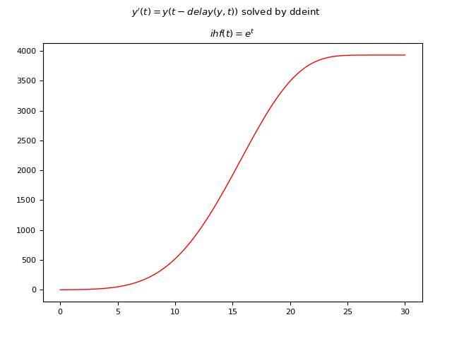
Graph of the numerical solution of the DDE obtained by ddeint.
JiTCDDE
Below is an example of Python code that numerically solves the DDE using JiTCDDE:
import numpy as np
import matplotlib.pyplot as plt
from jitcdde import jitcdde, y, t

def delay(y, t):
    return np.abs(0.1 * t * y(0, 0.1 * t))

equation = [y(0, t - delay(y, t))]
dde = jitcdde(equation, max_delay=1000)

def initial_history_func_exp_pt(t):
    return [np.exp(t)]

plt.rcParams['font.size'] = 8
fig, axs = plt.subplots(1, 1)
fig.tight_layout(rect=[0, 0, 1, 0.95], pad=3.0)
fig.suptitle("$y'(t)=y(t-delay(y, t))$ solved by jitcdde")

ts = np.linspace(0, 30, 10000)

dde.past_from_function(initial_history_func_exp_pt)
ys = []
for t in ts:
	ys.append(dde.integrate(t))
axs.plot(ts, ys, color='red', linewidth=1)
axs.set_title('$ihf(t)=e^t$')

plt.show()
Graph of the numerical solution of the DDE obtained by JiTCDDE.
Example #5: First-order DDE with two constant delays and a constant initial history function
Let the following DDE be given: $$ y'(t)=-y(t - 1) + 0.3 y(t - 2)$$ where the delays are two and are both constants equal to $1 s$ and $2 s$ respectively; The initial historical function is also constant and is $\phi(t)=1$.
ddeint
Below is an example of Python code that numerically solves the DDE using ddeint:
import numpy as np
import matplotlib.pyplot as plt
from ddeint import ddeint

def equation(Y, t):
    return -Y(t - 1) + 0.3 * Y(t - 2)

def initial_history_func(t):
    return 1.

plt.rcParams['font.size'] = 8
fig, axs = plt.subplots(1, 1)
fig.tight_layout(rect=[0, 0, 1, 0.95], pad=3.0)
fig.suptitle("$y'(t)=-y(t-1) + 0.3\ y(t-2)$ solved by ddeint")

ts = np.linspace(0, 10, 10000)

ys = ddeint(equation, initial_history_func, ts)
axs.plot(ts, ys, color='red', linewidth=1)
axs.set_title('$ihf(t)=1$')

plt.show()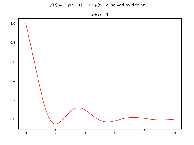
Graph of the numerical solution of the DDE obtained by ddeint.
JiTCDDE
Below is an example of Python code that numerically solves the DDE using JiTCDDE:
import numpy as np
import matplotlib.pyplot as plt
from jitcdde import jitcdde, y, t

equation=[-y(0, t - 1) + 0.3 * y(0, t - 2)]
dde = jitcdde(equation)

plt.rcParams['font.size'] = 8
fig, axs = plt.subplots(1, 1)
fig.tight_layout(rect=[0, 0, 1, 0.95], pad=3.0)
fig.suptitle("$y'(t)=-y(t-1) + 0.3\ y(t-2)$ solved by jitcdde")

ts = np.linspace(0, 10, 10000)

dde.constant_past([1.])
ys = []
for t in ts:
	ys.append(dde.integrate(t))
axs.plot(ts, ys, color='red', linewidth=1)
axs.set_title('$ihf(t)=1$')

plt.show()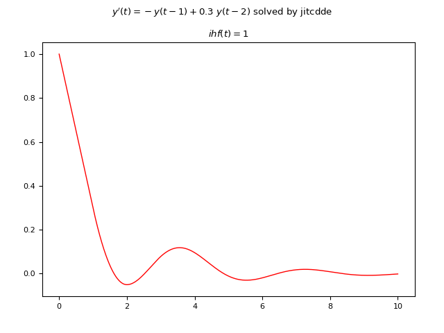
Graph of the numerical solution of the DDE obtained by JiTCDDE.
Example #6: System of two first-order DDEs with one constant delay and two constant initial history functions
Let the following system of DDEs be given: $$ \begin{equation} \begin{cases} y_1'(t) = y_1(t) y_2(t-0.5) \\ y_2'(t) = y_2(t) y_1(t-0.5) \end{cases} \end{equation} $$ where the delay is only one, constant and equal to $0.5 s$ and the initial historical functions are also constant; for what we said at the beginning of the post these must be two, in fact being the order of the system of first degree you need one for each unknown and they are: $y_1(t)=1, y_2(t)=-1$.
ddeint
Below is an example of Python code that numerically solves the DDE using ddeint:
import numpy as np
import matplotlib.pyplot as plt
from ddeint import ddeint

def equation(Y, t, d):
    x,y = Y(t)
    xd,yd = Y(t-d)
    return [x * yd, y * xd]

def initial_history_func(t):
    return [1., -1.]

plt.rcParams['font.size'] = 8
fig, axs = plt.subplots(1, 1)
fig.tight_layout(rect=[0, 0, 1, 0.95], pad=3.0)
fig.suptitle("$x'(t)=x(t) y(t-d); y'(t)=y(t) x(t-d)$ solved by ddeint")

ts = np.linspace(0, 3, 2000)

ys = ddeint(equation, initial_history_func, ts, fargs=(0.5,))
axs.plot(ts, ys[:,0], color='red', linewidth=1)
axs.plot(ts, ys[:,1], color='blue', linewidth=1)
axs.set_title('$ihf_x(t)=1; ihf_y(t)=-1; d=0.5$')

plt.show()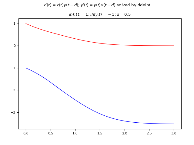
Graph of the numerical solution of the system of DDEs obtained by ddeint.
JiTCDDE
Below is an example of Python code that numerically solves the DDE using JiTCDDE:
import numpy as np
import matplotlib.pyplot as plt
import symengine
from jitcdde import jitcdde, y, t

d=symengine.symbols("d")
equations=[
	y(0, t) * y(1, t-d),
	y(1, t) * y(0, t-d)]
ddesys = jitcdde(equations, control_pars=[d], max_delay=100.)

plt.rcParams['font.size'] = 8
fig, axs = plt.subplots(1, 1)
fig.tight_layout(rect=[0, 0, 1, 0.95], pad=3.0)
fig.suptitle("$x'(t)=x(t) y(t-d); y'(t)=y(t) x(t-d)$ solved by jitcdde")

ts = np.linspace(0, 3, 2000)

ddesys.constant_past([1., -1.])
params=[0.5]
ddesys.set_parameters(*params)
ys = []
for t in ts:
	ys.append(ddesys.integrate(t))
ys=np.array(ys)
axs.plot(ts, ys[:,0], color='red', linewidth=1)
axs.plot(ts, ys[:,1], color='blue', linewidth=1)
axs.set_title('$ihf_x(t)=1; ihf_y(t)=-1; d=0.5$')

plt.show()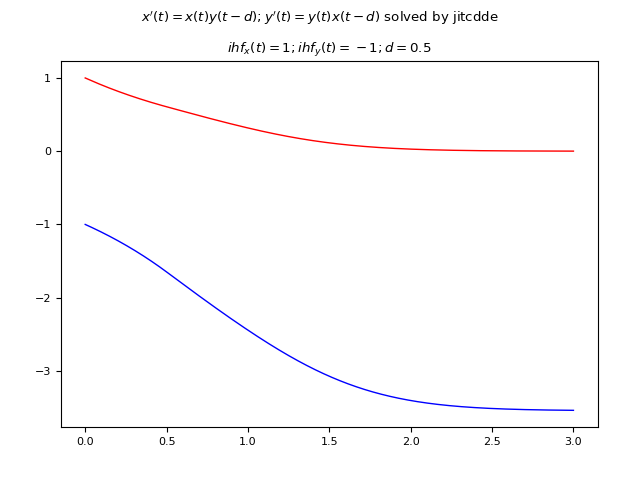
Graph of the numerical solution of the system of DDEs obtained by JiTCDDE.
Example #7: Second-order DDE with one constant delay and two constant initial history functions
Let the following DDE be given:
$$ y(t)'' = -y'(t) - 2y(t) - 0.5 y(t-1) $$
where the delay is only one, constant and equal to $1 s$.
Since the DDE is second order, in that the second derivative of the unknown function appears,
the historical functions must be two, one to give the values of the unknown $y(t)$ for $t <= 0$ and one
and one to provide the value of the first derivative $y'(t)$ also for $t <= 0$.
In this example they are the following two constant functions: $y(t)=1, y'(t)=0$.
Due to the properties of the second-order equations, the given DDE is equivalent to the following system of first-order equations:
$$ \begin{equation}
\begin{cases}
y_1'(t) = y_2(t)
\\
y_2'(t) = -y_1'(t) - 2y_1(t) - 0.5 y_1(t-1)
\end{cases}
\end{equation} $$
and so the implementation falls into the case of the previous example of systems of first-order equations.
ddeint
Below is an example of Python code that numerically solves the DDE using ddeint:
import numpy as np
import matplotlib.pyplot as plt
from ddeint import ddeint

def equation(Y, t):
    y,dydt = Y(t)
    ydelay, dydt_delay = Y(t-1)
    return [dydt, -dydt - 2 * y - 0.5 * ydelay]

def initial_history_func(t):
    return [1., 0.]

plt.rcParams['font.size'] = 8
fig, axs = plt.subplots(1, 1)
fig.tight_layout(rect=[0, 0, 1, 0.95], pad=3.0)
fig.suptitle("$y''(t)=-y'(t) - 2 y(t) - 0.5 y(t-1)$ solved by ddeint")

ts = np.linspace(0, 16, 4000)

ys = ddeint(equation, initial_history_func, ts)
axs.plot(ts, ys[:,0], color='red', linewidth=1)
#axs.plot(ts, ys[:,1], color='green', linewidth=1)
axs.set_title('$ihf_y(t)=1; ihf_dy/dt(t)=0$')

plt.show()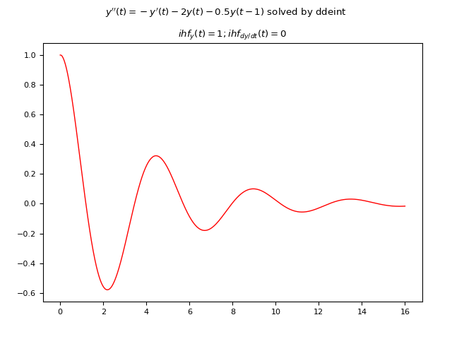
Graph of the numerical solution of the second-order DDE obtained by ddeint.
JiTCDDE
Below is an example of Python code that numerically solves the DDE using JiTCDDE:
import numpy as np
import matplotlib.pyplot as plt
from jitcdde import jitcdde, y, t

equations=[
    y(1, t),
    -y(1, t) - 2 * y(0, t) - 0.5 * y(0, t-1)
]
ddesys = jitcdde(equations)

plt.rcParams['font.size'] = 8
fig, axs = plt.subplots(1, 1)
fig.tight_layout(rect=[0, 0, 1, 0.95], pad=3.0)
fig.suptitle("$y''(t)=-y'(t) - 2 y(t) - 0.5 y(t-1)$ solved by jitcdde")

ts = np.linspace(0, 16, 4000)

ddesys.constant_past([1., 0.])
ys = []
for t in ts:
	ys.append(ddesys.integrate(t))
ys=np.array(ys)
axs.plot(ts, ys[:,0], color='red', linewidth=1)
#axs.plot(ts, ys[:,1], color='green', linewidth=1)
axs.set_title('$ihf_y(t)=1; ihf_dy/dt(t)=0$')

plt.show()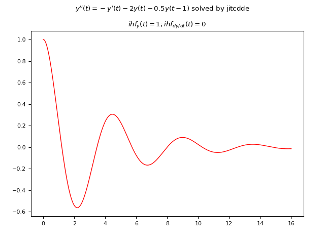
Graph of the numerical solution of the second-order DDE obtained by JiTCDDE.
Download of the complete code
The complete code is available at GitHub.
These materials are distributed under MIT license; feel free to use, share, fork and adapt these materials as you see fit.
Also please feel free to submit pull-requests and bug-reports to this GitHub repository or contact me on my social media channels available on the top right corner of this page.