Two-variables real-valued function fitting with PyTorch
This post is part of a series of posts on the fitting of mathematical objects (functions, curves and surfaces) through a MLP (Multi-Layer Perceptron) neural network;
for an introduction on the subject please see the post Fitting with highly configurable multi layer perceptrons.
The topic of this post is the fitting of a continuous and limited real-valued function of two variables constrained in a rectangle $$f(x,y) \colon [a,b]\times[c,d] \to \rm I\!R$$ with a MLP
so that the user can test different combinations of MLP architectures, their own activation functions, training algorithm and loss function without writing code
but working only on the command line of the four Python scripts which separately implement the following features:
- Dataset generation
- MLP architecture definition + Training
- Prediction
- Visualization of the result
To get the code please see the paragraph Download of the complete code at the end of this post.
The exact same mechanism was created using TensorFlow (with Keras) technology; see the post Two-variables real-valued function fitting with TensorFlow always published on this website.
If you are interested in regression of a real function of two variables with machine learning techniques see the post Fitting functions with a configurable XGBoost regressor.
Dataset generation
Goal of the fxy_gen.py Python program
is to generate datasets (both training and test ones) to be used in later phases;
it takes in command line the function of two variables to be approximated (in lambda body syntax), the rectangular subset of domain (specifing the two intervals of the sides of the rectangle) and discretization step
and it generates the dataset in an output csv file applying the function to the passed rectangle.
In fact the output csv file has three columns (without header): first two columns contain the values of independent variables $x$ and $y$ within the passed rectangle discretized by discretization step;
thrid column contains the values of dependent variable, ie the values of function $f(x,y)$ correspondent to values of $x$ and $y$ of first two columns.
To get the program usage you can run this following command:
$ python fxy_gen.py --helpusage: fxy_gen.py [-h]
-h, --help show this help message and exit
--dsout DS_OUTPUT_FILENAME dataset output file (csv format)
--fxy FUNC_X_BODY f(x,y) body (body lamba format)
--rxbegin RANGE_BEGIN begin x range (default:-5.0)
--rxend RANGE_END end x range (default:+5.0)
--rybegin RANGE_BEGIN begin y range (default:-5.0)
--ryend RANGE_END end y range (default:+5.0)
--rstep RANGE_STEP step range (default: 0.01)An example of using the program fxy_gen.py
Suppose you want to approximate in the rectagle $[-5.0,5.0]\times[-5.0,5.0]$ the function $$\sin \sqrt{x^2 + y^2}$$. Keeping in mind that np is the alias of NumPy library, the translation of this function in lambda body Python syntax is:
np.sin(np.sqrt(x**2 + y**2))$ python fxy_gen.py \
--dsout mytrain.csv \
--fxy "np.sin(np.sqrt(x**2 + y**2))" \
--rxbegin -5.0 \
--rxend 5.0 \
--rybegin -5.0 \
--ryend 5.0 \
--rstep 0.075$ python fxy_gen.py \
--dsout mytest.csv \
--fxy "np.sin(np.sqrt(x**2 + y**2))" \
--rxbegin -5.0 \
--rxend 5.0 \
--rybegin -5.0 \
--ryend 5.0 \
--rstep 0.275MLP architecture definition + Training
Goal of the fxy_fit.py Python program
is to dynamically create a MLP and perform its training according to the passed parameters through the command line.
To get the program usage you can run this following command:
$ python fxy_fit.py --helpusage: fxy_fit.py [-h]
--trainds TRAIN_DATASET_FILENAME
--modelout MODEL_PATH
[--epochs EPOCHS]
[--batch_size BATCH_SIZE]
[--hlayers HIDDEN_LAYERS_LAYOUT [HIDDEN_LAYERS_LAYOUT ...]]
[--hactivations ACTIVATION_FUNCTIONS [ACTIVATION_FUNCTIONS ...]]
[--optimizer OPTIMIZER]
[--loss LOSS]
[--device DEVICE]An example of using the program fxy_fit.py
Suppose you have a training dataset available (for example generated through fxy_gen.py program as shown in the previous paragraph)
and you want the MLP to have two hidden layers with both 100 neurons and that you want to use the ReLU activation function output from all two layers;
moreover you want to perform 10 training epochs with a 50 items batch size using the SGD optimizator algorithm with learning rate equal to 0.01,
momentum equal to 0.9, decay equal to 10-6 and nesterov flag set to true and loss function equal to MeanSquaredError.
To put all this into action, run the following command:
$ python fxy_fit.py \
  --trainds mytrain.csv \
  --modelout mymodel.pth \
  --hlayers 100 100 \
  --hactivations 'ReLU()' 'ReLU()' \
  --epochs 10 \
  --batch_size 50 \
  --optimizer 'SGD(lr=0.01, weight_decay=1e-6, momentum=0.9, nesterov=True)' \
--loss 'MeanSquaredError()'mymodel.pth will contain the MLP model trained on mytrain.csv dataset according to the parameters passed on the command line.
Prediction
Goal of the fxy_predict.py Python program
is to apply the MLP model generated through fxy_fit.py to an input dataset (for example the test dataset generated through fxy_gen.py program as shown in a previous paragraph);
the execution of the program produces in output a csv file with three columns (without header): the first two columns contains the values of indepedent variable $x$ and $y$ taken from test dataset
and the third column contains the predicted values of dependent variable, ie the values of the prediction correspondent to values of $x$ and $y$ of first two columns.
To get the program usage you can run this following command:
$ python fxy_predict.py --helpusage: fxy_predict.py [-h]
--model MODEL_PATH
--ds DATASET_FILENAME
--predictionout PREDICTION_DATA_FILENAME
[--device DEVICE]An example of using the program fxy_predict.py
Suppose you have the test dataset mytest.csv available (for example generated through fxy_gen.py program as shown in a previous paragraph)
and the trained model of MLP in the file mymodel.pth (generated through fxy_fit.py program as shown in the example of previous paragraph); run the following command:
$ python fxy_predict.py \
  --model mymodel.pth \
  --ds mytest.csv \
  --predictionout myprediction.csv
myprediction.csv will contain the fitting of the initial function.
Visualization of the result
Goal of the fxy_plot.py Python program
is to visualize the prediction curve superimposed on initial dataset curve (test or training, as you prefer) and it allows the visual comparison of the two curves.
To get the program usage you can run this following command:
$ python fxy_plot.py --helpusage: fxy_plot.py [-h]
--ds DATASET_FILENAME
--prediction PREDICTION_DATA_FILENAME
[--savefig SAVE_FIGURE_FILENAME]An example of using the program fxy_plot.py
Having the test dataset mytest.csv available (for example generated through fxy_gen.py program as shown in a previous paragraph)
and the prediction csv file (generated through fxy_predict.py program as shown in the previous paragraph), to generate the two xy-scatter charts, execute the following command:
$ python fxy_plot.py \
  --ds mytest.csv \
--prediction myprediction.csvNote: Given the stochastic nature of the training phase, your specific results may vary. Consider running the example a few times.
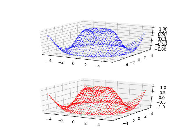
Chart generated by the program
fxy_plot.py that shows the fitting of the function $f(x)=\frac{\sin 2x}{e^\frac{x}{5}}$ made by the MLP.Examples of cascade use of the four programs
In the folder two-variables-function-fitting/examples
there are three shell scripts that show the use in cascade of the four programs in various combinations of parameters
(MLP architecture, activation functions, optimization algorithm, loss function, training procedure parameters)
To run the three examples, run the following commands:
$ cd two-variables-function-fitting/examples
$ sh example1.sh
$ sh example2.sh
$ sh example3.shDownload of the complete code
The complete code is available at GitHub.
These materials are distributed under MIT license; feel free to use, share, fork and adapt these materials as you see fit.
Also please feel free to submit pull-requests and bug-reports to this GitHub repository or contact me on my social media channels available on the top right corner of this page.