Common tools for function fitting
This post describes the use of a set of common tools written in Python to generate and display synthetic datasets
obtained by performing both scalar and vector generator functions of one or more variables
or datasets obtained by approximating such functions through appropriate programs described in other posts on this website
that deal with the fitting of mathematical objects (functions, curves and surfaces) both with machine learning algorithms and neural networks.
The areas affected by these tools are:
- Creation of synthetic datasets
- Comparative display of datasets
- Diagnostics
To get the code of each tool follow the link at the beginning of each paragraph related to the tool itself; the paragraph Download of the complete code contains the link to the entire repository which deals with the approximation of mathematical functions with machine and deep learning techniques.
Creation of synthetic datasets
This chapter explains the tools for generating synthetic datasets from mathematical generator functions.
fx_gen.py
Goal of the fx_gen.py Python program
is to generate a synthetic dataset in csv format starting from a real-valued and scalar generator function of a real-valued variable in a closed interval specifying the step of discretization.
The output csv file has two columns (with header): first column contains the sorted values of independent variable $x$ within the passed interval discretized by discretization step;
second column contains the values of dependent variable, ie the values of function $f(x)$ correspondent to values of $x$ of first column.
To get the program usage you can run this following command:
$ python fx_gen.py --helpusage: fx_gen.py [-h] [--version] --dsout DS_OUTPUT_FILENAME --funcx
FUNC_X_BODY [--xbegin RANGE_BEGIN] [--xend RANGE_END]
[--xstep RANGE_STEP] [--noise NOISE_BODY]
fx_gen.py generates a synthetic dataset file calling a one-variable real
function in an interval
optional arguments:
-h, --help show this help message and exit
--version show program's version number and exit
--dsout DS_OUTPUT_FILENAME
dataset output file (csv format)
--funcx FUNC_X_BODY f(x) body (lamba format)
--xbegin RANGE_BEGIN begin range (default:-5.0)
--xend RANGE_END end range (default:+5.0)
--xstep RANGE_STEP step range (default: 0.01)
--noise NOISE_BODY noise(sz) body (lamba format)-
-h, --help: shows the usage of the program and ends the execution.
-
--version: shows the version of the program and ends the execution.
-
--dsout: path (relative or absolute) of the csv file to be generated and got executing the dataset generator function.
-
--funcx: the generator function $y=f(x)$ of the time dataset in lamba body format where $x$ is the independent variable.
-
--xbegin e --xend: the closed interval of the variable $x$, between
--xbeginand--xend.
-
--xstep: the discretization step of the independent variable $x$.
-
--noise: the noise generator functon lamba body format,
where $sz$ is the number of elements of the discretized interval between
--xbeginand--xend.
An example of using the fx_gen.py program
Suppose you want to approximate the function $$f(x)=\sqrt{|x|}$$ in the range $[-6.0,6.0]$ Keeping in mind that np is the alias of NumPy library, the translation of this function in lambda body Python syntax is:
np.sqrt(np.abs(x))$ python fx_gen.py \
--dsout mytrain.csv \
--funcx "np.sqrt(np.abs(x))" \
--xbegin -6.0 \
--xend 6.0 \
--xstep 0.01fxy_gen.py
Goal of the fxy_gen.py Python program
is to generate a synthetic dataset in csv format starting from a real-valued and scalar generator function of two real-valued variables in a closed rectangle specifying the step of discretization.
The output csv file has three columns (with header): first two columns contain the sorted values of independent variables $x$ and $y$ within the passed intervals discretized by their own discretization steps;
third column contains the values of dependent variable, ie the values of function $f(x,y)$ correspondent to values of $x$ and $y$ of first two columns.
To get the program usage you can run this following command:
$ python fxy_gen.py --helpusage: fxy_gen.py [-h] [--version] --dsout DS_OUTPUT_FILENAME --funcxy
FUNC_XY_BODY [--xbegin RANGE_XBEGIN] [--xend RANGE_XEND]
[--ybegin RANGE_YBEGIN] [--yend RANGE_YEND]
[--xstep RANGE_XSTEP] [--ystep RANGE_YSTEP]
[--noise NOISE_BODY]
fxy_gen.py generates a synthetic dataset file calling a two-variables real
function on a rectangle
optional arguments:
-h, --help show this help message and exit
--version show program's version number and exit
--dsout DS_OUTPUT_FILENAME
dataset output file (csv format)
--funcxy FUNC_XY_BODY
f(x, y) body (lamba format)
--xbegin RANGE_XBEGIN
begin x range (default:-5.0)
--xend RANGE_XEND end x range (default:+5.0)
--ybegin RANGE_YBEGIN
begin y range (default:-5.0)
--yend RANGE_YEND end y range (default:+5.0)
--xstep RANGE_XSTEP step range of x (default: 0.01)
--ystep RANGE_YSTEP step range of y (default: 0.01)
--noise NOISE_BODY noise(sz) body (lamba format)-
-h, --help: shows the usage of the program and ends the execution.
-
--version: shows the version of the program and ends the execution.
-
--dsout: path (relative or absolute) of the csv file to be generated and got executing the dataset generator function.
-
--funcxy: the generator function $y=f(x,y)$ of the time dataset in lamba body format where $x$ and $y$ are the independent variables.
-
--xbegin e --xend: the closed interval of the variable $x$, between
--xbeginand--xend.
-
--ybegin e --yend: the closed interval of the variable $y$, between
--ybeginand--yend.
-
--xstep: the discretization step of the independent variable $x$.
-
--ystep: the discretization step of the independent variable $y$.
-
--noise: the noise generator functon lamba body format,
where $sz$ is the number of elements of the discretized rectagle between
--xbeginand--xendfor--ybeginand--yend. interval between--xbeginand--xend.
An example of using the fxy_gen.py program
Suppose you want to approximate in the rectagle $[-6.0,6.0]\times[-6.0,6.0]$ the following function $$\sin \sqrt{x^2 + y^2}$$, Keeping in mind that np is the alias of NumPy library, the translation of this function in lambda body Python syntax is:
np.sin(np.sqrt(x**2 + y**2))$ python fxy_gen.py \
--dsout mytrain.csv \
--funcxy "np.sin(np.sqrt(x**2 + y**2))" \
--xbegin -6.0 \
--xend 6.0 \
--ybegin -6.0 \
--yend 6.0 \
--xstep 0.075 \
--ystep 0.075pmc2t_gen.py
Goal of the pmc2t_gen.py Python program
is to generate a synthetic dataset in csv format starting from a couple of real-valued functions of one real-valued variable $t$, called parameter:
it takes in command line the two component functions to be approximated (in lambda body syntax), the interval of independent parameter $t$ (begin, end and discretization step)
and it generates the dataset in an output csv file applying the two functions to the passed interval of the parameter $t$.
In fact the output csv file has three columns (with header): first column contains the sorted values of independent parameter $t$ within the passed interval discretized by discretization step;
second and third columns contain respectively the values of the components $x$ and $y$, ie the values of functions $x(t)$ and $y(t)$ correspondent to values of $t$ of first column.
To get the program usage you can run this following command:
$ python pmc2t_gen.py --helpusage: pmc2t_gen.py [-h] [--version] --dsout DS_OUTPUT_FILENAME --funcxt
FUNCX_T_BODY --funcyt FUNCY_T_BODY [--tbegin RANGE_BEGIN]
[--tend RANGE_END] [--tstep RANGE_STEP]
[--xnoise XNOISE_BODY] [--ynoise YNOISE_BODY]
pmc2t_gen.py generates a synthetic dataset file that contains the points of a
parametric curve on plane calling a couple of one-variable real functions in
an interval
optional arguments:
-h, --help show this help message and exit
--version show program's version number and exit
--dsout DS_OUTPUT_FILENAME
dataset output file (csv format)
--funcxt FUNCX_T_BODY
x=x(t) body (lamba format)
--funcyt FUNCY_T_BODY
y=y(t) body (lamba format)
--tbegin RANGE_BEGIN begin range (default:-5.0)
--tend RANGE_END end range (default:+5.0)
--tstep RANGE_STEP step range (default: 0.01)
--xnoise XNOISE_BODY noise(sz) body (lamba format) on x
--ynoise YNOISE_BODY noise(sz) body (lamba format) on y-
-h, --help: shows the usage of the program and ends the execution.
-
--version: shows the version of the program and ends the execution.
-
--dsout: path (relative or absolute) of the csv file to be generated and got executing the dataset generator function.
-
--funcxt: the generator function $x=fx(t)$ of the time dataset in lamba body format where $t$ is the independent variable.
-
--funcyt: the generator function $y=fy(t)$ of the time dataset in lamba body format where $t$ is the independent variable.
-
--tbegin e --tend: the closed interval of the variable $t$, between
--tbeginand--tend.
-
--tstep: the discretization step of the independent variable $x$.
-
--xnoise: the noise generator functon on $x$ variable in lamba body format,
where $sz$ is the number of elements of the discretized interval between
--tbeginand--tend.
-
--ynoise: the noise generator functon on $y$ variable in lamba body format,
where $sz$ is the number of elements of the discretized interval between
--tbeginand--tend.
pmc3t_gen.py
Goal of the pmc3t_gen.py Python program
is to generate a synthetic dataset in csv format starting from a triple of real-valued functions of one real-valued variable $t$, called parameter
it takes in command line the three component functions to be approximated (in lambda body syntax), the interval of independent parameter $t$ (begin, end and discretization step)
and it generates the dataset in an output csv file applying the three functions to the passed interval of the parameter $t$.
In fact the output csv file has four columns (with header): first column contains the sorted values of independent parameter $t$ within the passed interval discretized by discretization step;
second, third and fourth columns contain respectively the values of the components $x$, $y$ and $z$, ie the values of functions $x(t)$, $y(t)$ and $z(t)$ correspondent to values of $t$ of first column.
To get the program usage you can run this following command:
$ python pmc3t_gen.py --helpusage: pmc3t_gen.py [-h] [--version] --dsout DS_OUTPUT_FILENAME --funcxt
FUNCX_T_BODY --funcyt FUNCY_T_BODY --funczt FUNCZ_T_BODY
[--tbegin RANGE_BEGIN] [--tend RANGE_END]
[--tstep RANGE_STEP] [--xnoise XNOISE_BODY]
[--ynoise YNOISE_BODY] [--znoise ZNOISE_BODY]
pmc3t_gen.py generates a synthetic dataset file that contains the points of a
parametric curve in space calling a a triple of one-variable real functions in
an interval
optional arguments:
-h, --help show this help message and exit
--version show program's version number and exit
--dsout DS_OUTPUT_FILENAME
dataset output file (csv format)
--funcxt FUNCX_T_BODY
x=x(t) body (lamba format)
--funcyt FUNCY_T_BODY
y=y(t) body (lamba format)
--funczt FUNCZ_T_BODY
z=z(t) body (lamba format)
--tbegin RANGE_BEGIN begin range (default:-5.0)
--tend RANGE_END end range (default:+5.0)
--tstep RANGE_STEP step range (default: 0.01)
--xnoise XNOISE_BODY noise(sz) body (lamba format) on x
--ynoise YNOISE_BODY noise(sz) body (lamba format) on y
--znoise ZNOISE_BODY noise(sz) body (lamba format) on z-
-h, --help: shows the usage of the program and ends the execution.
-
--version: shows the version of the program and ends the execution.
-
--dsout: path (relative or absolute) of the csv file to be generated and got executing the dataset generator function.
-
--funcxt: the generator function $x=fx(t)$ of the time dataset in lamba body format where $t$ is the independent variable.
-
--funcyt: the generator function $y=fy(t)$ of the time dataset in lamba body format where $t$ is the independent variable.
-
--funcyt: the generator function $z=fz(t)$ of the time dataset in lamba body format where $t$ is the independent variable.
-
--tbegin e --tend: the closed interval of the variable $t$, between
--tbeginand--tend.
-
--tstep: the discretization step of the independent variable $x$.
-
--xnoise: the noise generator functon on $x$ variable in lamba body format,
where $sz$ is the number of elements of the discretized interval between
--tbeginand--tend.
-
--ynoise: the noise generator functon on $y$ variable in lamba body format,
where $sz$ is the number of elements of the discretized interval between
--tbeginand--tend.
-
--znoise: the noise generator functon on $z$ variable in lamba body format,
where $sz$ is the number of elements of the discretized interval between
--tbeginand--tend.
Comparative display of datasets
This chapter explains the tools for viewing datasets allowing to visually compare the input datasets with the prediction generated by the approximators.
fx_scatter.py
Goal of the fx_scatter.py Python program
is to display the scatter graph of the prediction of a real-valued scalar function of a real-valued variable
superimposed on the scatter graph of the input dataset of the original function and allow the visual comparison of the two graphs.
To get the program usage you can run this following command:
$ python fx_scatter.py --helpusage: fx_scatter.py [-h] [--version] --ds DATASET_FILENAME --prediction
PREDICTION_DATA_FILENAME [--title FIGURE_TITLE]
[--xlabel X_AXIS_LABEL] [--ylabel Y_AXIS_LABEL]
[--labelfontsize LABEL_FONT_SIZE] [--width WIDTH]
[--height HEIGHT] [--savefig SAVE_FIGURE_FILENAME]
fx_scatter.py shows two overlapped x/y scatter graphs: the blue one is the
input dataset, the red one is the prediction
optional arguments:
-h, --help show this help message and exit
--version show program's version number and exit
--ds DATASET_FILENAME
dataset file (csv format)
--prediction PREDICTION_DATA_FILENAME
prediction data file (csv format)
--title FIGURE_TITLE if present, it set the title of chart
--xlabel X_AXIS_LABEL
label of x axis
--ylabel Y_AXIS_LABEL
label of y axis
--labelfontsize LABEL_FONT_SIZE
label font size
--width WIDTH width of whole figure (in inch)
--height HEIGHT height of whole figure (in inch)
--savefig SAVE_FIGURE_FILENAME
if present, the figure is saved on a file instead to be
shown on screen-
-h, --help: shows the usage of the program and ends the execution.
-
--version: shows the version of the program and ends the execution.
-
--ds: path (relative or absolute) to input dataset file; the color of its related scatter graph is blue.
-
--prediction: path (relative or absolute) to prediction file (always in csv format); the color of its related scatter graph is red.
-
--title: title of the figure, centered at the top.
-
--xlabel: $x$ axis caption.
-
--ylabel: $y$ axis caption.
-
--labelfontsize: sets the font of the texts in the figure.
-
--width: sets the width of the generated figure, in inch
-
--height: sets the height of the generated figure, in inch
-
--savefig:
if it is present, it is the path (relative or absolute) of the figure file in .png format to be saved;
if not present, the graph is shown on screen in a window.
An example of using the fx_scatter.py program
Having available the mytest.csv test dataset (for example generated via fx_gen.py as shown in a previous paragraph)
and the mypred.csv prediction csv file (generated through a prediction program in the repository for the fitting of functions of one variable),
to generate the two graphs, run the following command:
$ python fx_scatter.py \
  --ds mytest.csv \
  --prediction mypred.csv \
  --title "My example" \
  --xlabel "x" \
  --ylabel "y=|sin(x^x)/2^(x^x-pi/2)/pi|"
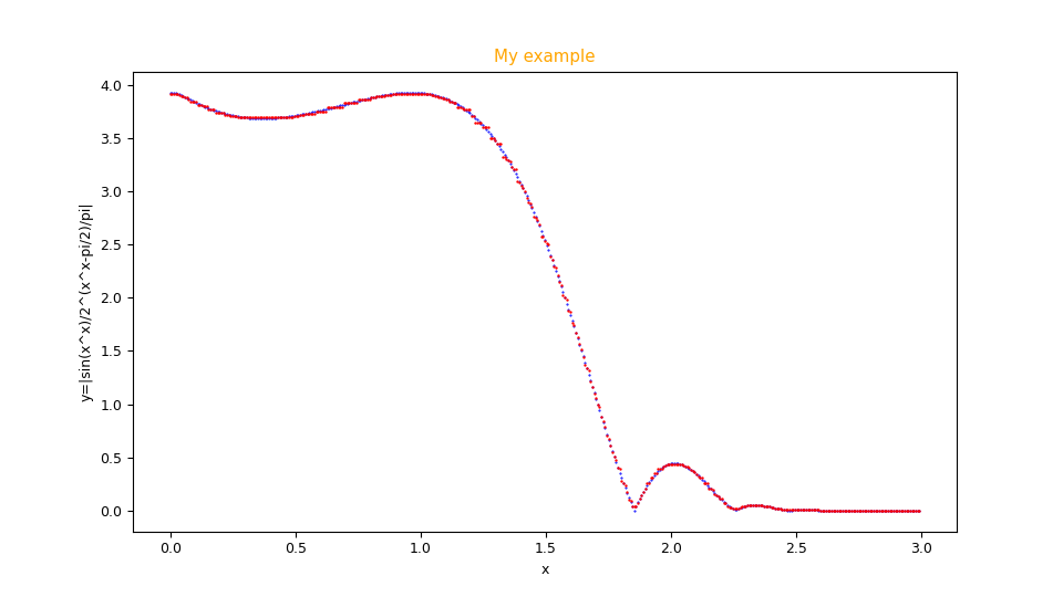
Figure with scatter graphics generated by the program
fx_scatter.py showing the fitting in red overlay of the function $f(x)=|\frac{\sin x^x}{2 ^ {(x^x - \pi/2)/\pi}}|$
and the original function below in blue.fxy_scatter.py
Goal of the fxy_scatter.py Python program
is to display the scatter graph of the prediction of a real-valued scalar function of two real-valued variables
alongside the scatter graph of the input dataset of the original function and allow the visual comparison of the two graphs.
To get the program usage you can run this following command:
$ python fxy_scatter.py --helpusage: fxy_scatter.py [-h] [--version] --ds DATASET_FILENAME --prediction
PREDICTION_DATA_FILENAME [--title FIGURE_TITLE]
[--xlabel X_AXIS_LABEL] [--ylabel Y_AXIS_LABEL]
[--zlabel Z_AXIS_LABEL]
[--labelfontsize LABEL_FONT_SIZE] [--width WIDTH]
[--height HEIGHT] [--savefig SAVE_FIGURE_FILENAME]
fxy_scatter.py: error: the following arguments are required: --ds, --prediction
(base) malkuth:common ettore$ python fxy_scatter.py --help
usage: fxy_scatter.py [-h] [--version] --ds DATASET_FILENAME --prediction
PREDICTION_DATA_FILENAME [--title FIGURE_TITLE]
[--xlabel X_AXIS_LABEL] [--ylabel Y_AXIS_LABEL]
[--zlabel Z_AXIS_LABEL]
[--labelfontsize LABEL_FONT_SIZE] [--width WIDTH]
[--height HEIGHT] [--savefig SAVE_FIGURE_FILENAME]
fxy_scatter.py shows two alongside x/y/z scatter graphs: the blue one is the
surface of dataset, the red one is the surface of prediction
optional arguments:
-h, --help show this help message and exit
--version show program's version number and exit
--ds DATASET_FILENAME
dataset file (csv format)
--prediction PREDICTION_DATA_FILENAME
prediction data file (csv format)
--title FIGURE_TITLE if present, it set the title of chart
--xlabel X_AXIS_LABEL
label of x axis
--ylabel Y_AXIS_LABEL
label of y axis
--zlabel Z_AXIS_LABEL
label of z axis
--labelfontsize LABEL_FONT_SIZE
label font size
--width WIDTH width of animated git (in inch)
--height HEIGHT height of animated git (in inch)
--savefig SAVE_FIGURE_FILENAME
if present, the chart is saved on a file instead to be
shown on screen-
-h, --help: shows the usage of the program and ends the execution.
-
--version: shows the version of the program and ends the execution.
-
--ds: path (relative or absolute) to input dataset file; the color of its related scatter graph is blue.
-
--prediction: path (relative or absolute) to prediction file (always in csv format); the color of its related scatter graph is red.
-
--title: title of the figure, centered at the top.
-
--xlabel: $x$ axis caption.
-
--ylabel: $y$ axis caption.
-
--zlabel: $z$ axis caption.
-
--labelfontsize: sets the font of the texts in the figure.
-
--width: sets the width of the generated figure, in inch
-
--height: sets the height of the generated figure, in inch
-
--savefig:
if it is present, it is the path (relative or absolute) of the figure file in .png format to be saved;
if not present, the graph is shown on screen in a window.
An example of using the fxy_scatter.py program
Having available the mytest.csv test dataset (for example generated via fxy_gen.py as shown in a previous paragraph)
and the mypred.csv prediction csv file (generated through a prediction program in the repository for the fitting of functions of two variables),
to generate the two graphs, run the following command:
$ python fxy_scatter.py \
  --ds mytest.csv \
  --prediction mypred.csv \
  --title "My example" \
  --xlabel "x" \
  --ylabel "y" \
  --zlabel "z=2 sin(x)^2 / sqrt(1+y^2)"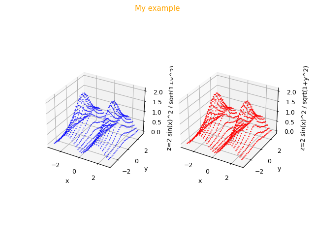
Figure with scatter graphics generated by the program
fxy_scatter.py showing the fitting to the right in red of the function $f(x,y)=2 \frac{\sin^2 x}{\sqrt{1 + y^2}}$
and alongside the graph of the original function to the left in blue.pmc2t_scatter.py
Goal of the pmc2t_scatter.py Python program
is to display the scatter graph of the prediction of a parametric curve on plane
overlapped the scatter graph of the input dataset of the original parametric curve and allow the visual comparison of the two graphs.
To get the program usage you can run this following command:
$ python pmc2t_scatter.py --helpusage: pmc2t_scatter.py [-h] [--version] --ds DATASET_FILENAME --prediction
PREDICTION_DATA_FILENAME [--title FIGURE_TITLE]
[--xlabel X_AXIS_LABEL] [--ylabel Y_AXIS_LABEL]
[--labelfontsize LABEL_FONT_SIZE] [--width WIDTH]
[--height HEIGHT] [--savefig SAVE_FIGURE_FILENAME]
pmc2t_scatter.py shows two overlapped x/y scatter graphs on plane: the blue
one is the input dataset of parametric curve, the red one is the prediction of
parametric curve
optional arguments:
-h, --help show this help message and exit
--version show program's version number and exit
--ds DATASET_FILENAME
dataset file (csv format)
--prediction PREDICTION_DATA_FILENAME
prediction data file (csv format)
--title FIGURE_TITLE if present, it set the title of chart
--xlabel X_AXIS_LABEL
label of x axis
--ylabel Y_AXIS_LABEL
label of y axis
--labelfontsize LABEL_FONT_SIZE
label font size
--width WIDTH width of whole figure (in inch)
--height HEIGHT height of whole figure (in inch)
--savefig SAVE_FIGURE_FILENAME
if present, the figure is saved on a file instead to
be shown on screen-
-h, --help: shows the usage of the program and ends the execution.
-
--version: shows the version of the program and ends the execution.
-
--ds: path (relative or absolute) to input dataset file; the color of its related scatter graph is blue.
-
--prediction: path (relative or absolute) to prediction file (always in csv format); the color of its related scatter graph is red.
-
--title: title of the figure, centered at the top.
-
--xlabel: $x$ axis caption.
-
--ylabel: $y$ axis caption.
-
--labelfontsize: sets the font of the texts in the figure.
-
--width: sets the width of the generated figure, in inch
-
--height: sets the height of the generated figure, in inch
-
--savefig:
if it is present, it is the path (relative or absolute) of the figure file in .png format to be saved;
if not present, the graph is shown on screen in a window.
pmc3t_scatter.py
Goal of the fxy_scatter.py Python program
is to display the scatter graph of the prediction of a parametric curve in space
overlapped the scatter graph of the input dataset of the original parametric curve and allow the visual comparison of the two graphs.
To get the program usage you can run this following command:
$ python pmc3t_scatter.py --help -h, --help show this help message and exit
--version show program&aposMs version number and exit
--ds DATASET_FILENAME
dataset file (csv format)
--prediction PREDICTION_DATA_FILENAME
prediction data file (csv format)
--title FIGURE_TITLE if present, it set the title of chart
--xlabel X_AXIS_LABEL
label of x axis
--ylabel Y_AXIS_LABEL
label of y axis
--zlabel Z_AXIS_LABEL
label of z axis
--labelfontsize LABEL_FONT_SIZE
label font size
--width WIDTH width of whole figure (in inch)
--height HEIGHT height of whole figure (in inch)
--savefig SAVE_FIGURE_FILENAME
if present, the figure is saved on a file instead to
be shown on screen
-
-h, --help: shows the usage of the program and ends the execution.
-
--version: shows the version of the program and ends the execution.
-
--ds: path (relative or absolute) to input dataset file; the color of its related scatter graph is blue.
-
--prediction: path (relative or absolute) to prediction file (always in csv format); the color of its related scatter graph is red.
-
--title: title of the figure, centered at the top.
-
--xlabel: $x$ axis caption.
-
--ylabel: $y$ axis caption.
-
--zlabel: $z$ axis caption.
-
--labelfontsize: sets the font of the texts in the figure.
-
--width: sets the width of the generated figure, in inch
-
--height: sets the height of the generated figure, in inch
-
--savefig:
if it is present, it is the path (relative or absolute) of the figure file in .png format to be saved;
if not present, the graph is shown on screen in a window.
Diagnostics
This chapter explains the diagnostic tools provided by this repository for the fitting of functions; the programs in this repository that implement the training features save (if the user so wishes) dump files usable later and/or during the training phase by the programs described herein with the aim of analyzing how the training phase has happened (or is happening) and then operate on the hyper parameters to improve the final result.
dumps_scatter.py
Goal of the dumps_scatter.py Phyton program
is to display the graphs of the loss function and the various metrics calculated during the training phase.
In order to be able to use this program it is necessary that the training programs have been launched
with the appropriate arguments to save the dump files of the loss function and/or metrics as the epochs change.
To get the program usage you can run this following command:
$ python dumps_scatter.py --helpusage: dumps_scatter.py [-h] [--version] --dump DUMP_PATH
[--savefigdir SAVE_FIGURE_DIRECTORY]
dumps_scatter.py shows the loss and metric graphs with data generated by
any fitting program with argument --dumpout
optional arguments:
-h, --help show this help message and exit
--version show program's version number and exit
--dump DUMP_PATH Dump directory (generated by any fitting/training
programs of this suite that support --dumpout
argument)
--savefigdir SAVE_FIGURE_DIRECTORY
If present, the charts are saved on files in
savefig_dir folder instead to be shown on screen-
-h, --help: shows the usage of the program and ends the execution.
-
--version: shows the version of the program and ends the execution.
-
--dump: path (relative or absolute) of the directory where the loss function and/or metrics dumps were saved during the training as the epochs change.
-
--savefigdir:
if it is present, it is the path (relative or absolute) of the directory where the program saves the figures in .png format, one figure for each graph for which the corresponding dump file exists;
if not present, the graphs are shown on screen.
An example of using the dumps_scatter.py program
Having available the directory mydumps which contains the dump files of some metrics calculated during the training phase
of some training program in this repository, to view the graphs of these metrics run the following command:
$ python dumps_scatter.py \
--dump mydumpsmydumps folder, as shown in the following figures.
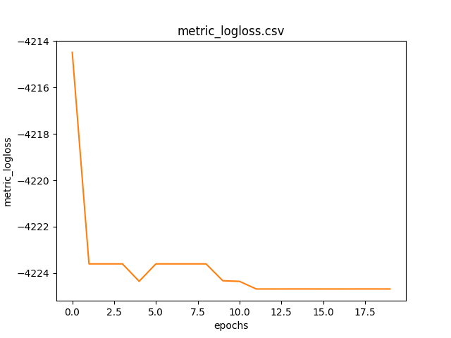
Graph of the metric logloss as the epochs change calculated on the training dataset.
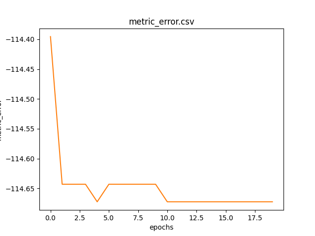
Graph of the metric error as the epochs change calculated on the training dataset.
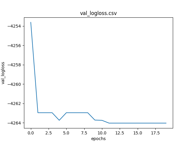
Graph of the metric logloss as the epochs change calculated on validation dataset.
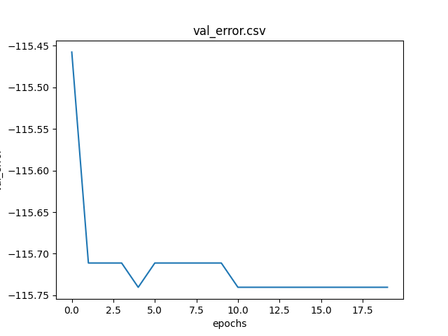
Graph of the metric error as the epochs change calculated on validation dataset.
Download of the complete code
The complete code is available at GitHub.
These materials are distributed under MIT license; feel free to use, share, fork and adapt these materials as you see fit.
Also please feel free to submit pull-requests and bug-reports to this GitHub repository or contact me on my social media channels available on the top right corner of this page.