Ordinary differential equation solvers in Python
This post shows the use of some ordinary differential equation (abbreviated ODE) solvers
implemented by libraries for Python frequently used in scientific applications in general and especially in machine learning and deep learning.
The resolution techniques shown here are numerical and not analytical techniques, as this site deals with computation.
Moreover this post is published under the category of neural networks: although not all the techniques shown here
use technologies of deep learning, its purpose is to be proactive to the topic on the relationship between neural networks and differential equations.
The post is organized as a sort of Rosetta Stele: three problems are presented
namely an equation of the first order, a system of two equations of the first order and an equation of the second order each with its own initial conditions
(or Cauchy's condition, abbreviated IVP for Initial Value Problem) and below the list of their solutions with the various libraries used.
Of each problem the analytical solution is also known and this allows to compare the quality of the numerical solutions obtained.
The Rosetta Stone continues in the post Ordinary differential equation solvers in Julia where it shows the solution of the same problems in Julia.
.
All the various code fragments described in this post require Python version 3 and the MatPlotLib and NumPy libraries
while individually require an additional library (and its own dependencies) in accordance with the solver used.
To get the code see paragraph Download the complete code at the end of this post.
Conventions
In this post the conventions used are as follows:
- $t$ is the independent variable
- $x$ is the unknown function
- $y$ is the second unknown function in the case of systems of two equations
- $x$ and $y$ are intended to be functions of $t$, so $x=x(t)$ and $y=y(t)$, but the use of this compact notation, in addition to having a greater readability at a mathematical level makes it easier to "translate" the equation into code
- $x'$ is the first derivative of $x$ with respect to $t$ and of course $y'$ is the first derivative of $y$ with respect to $t$
- $x''$ is the second derivative of $x$ with respect to $t$ and of course $y''$ is the second derivative of $y$ with respect to $t$
First order ODE with IVP
Let the following Cauchy problem be given:
$$ \begin{equation}
\begin{cases}
x'+x=\sin t + 3 \cos 2t
\\
x(0)=0
\end{cases}
\end{equation} $$
whose analytical solution is:
$$ x(t) = \frac{1}{2} \sin t − \frac{1}{2} \cos t + \frac{3}{5} \cos 2t + \frac{6}{5} \sin 2t − \frac{1}{10}e^{-t} $$
verifiable online via Wolfram Alpha.
Implementations of the following resolutions require the differential equation to be written explicitly in the form $x'=F(x,t)$
and then it becomes:
$$ x'=\sin t + 3 \cos 2t - x$$
Scipy
Scipy uses the scipy.integrate.solve_ivp function
to numerically solve an ordinary first order differential equation with initial value.
The explicit form of the above equation in Python with NumPy is implemented as follows:
lambda t, x: np.sin(t) + 3. * np.cos(2. * t) - xBelow is an example of Python code that compares the analytical solution with the numerical one obtained by
scipy.integrate.solve_ivp:
import numpy as np
import matplotlib.pyplot as plt

from scipy.integrate import solve_ivp

ode_fn = lambda t, x: np.sin(t) + 3. * np.cos(2. * t) - x

an_sol = lambda t : (1./2.) * np.sin(t) - (1./2.) * np.cos(t) + \
                    (3./5.) * np.cos(2.*t) + (6./5.) * np.sin(2.*t) - \
                    (1./10.) * np.exp(-t)
t_begin=0.
t_end=10.
t_nsamples=100
t_space = np.linspace(t_begin, t_end, t_nsamples)
x_init = 0.

x_an_sol = an_sol(t_space)

method = 'RK45' #available methods: 'RK45', 'RK23', 'DOP853', 'Radau', 'BDF', 'LSODA'
num_sol = solve_ivp(ode_fn, [t_begin, t_end], [x_init], method=method, dense_output=True)
x_num_sol = num_sol.sol(t_space).T

plt.figure()
plt.plot(t_space, x_an_sol, '--', linewidth=2, label='analytical')
plt.plot(t_space, x_num_sol, linewidth=1, label='numerical')
plt.title('ODE 1st order IVP solved by SciPy with method=' + method)
plt.xlabel('t')
plt.ylabel('x')
plt.legend()
plt.show()
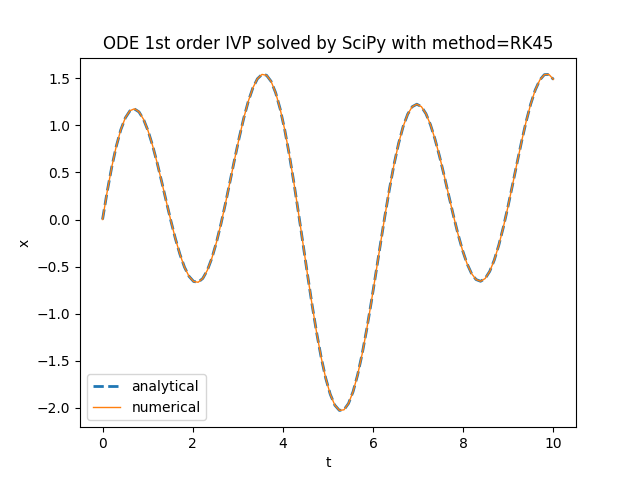
Comparison of the analytical solution with the numerical solution obtained by
scipy.integrate.solve_ivp.TensorFlow Probability
TensorFlow Probability uses the tfp.math.ode.BDF class
to numerically solve an ordinary first order differential equation with initial value.
The explicit form of the above equation in Python with TensorFlow Probability is implemented as follows:
lambda t, x: tf.math.sin(t) + tf.constant(3.) * tf.math.cos(tf.constant(2.) * t) - xBelow is an example of Python code that compares the analytical solution with the numerical one obtained by
tfp.math.ode.BDF:
import numpy as np
import matplotlib.pyplot as plt

import tensorflow as tf
import tensorflow_probability as tfp

ode_fn = lambda t, x: tf.math.sin(t) + tf.constant(3.) * tf.math.cos(tf.constant(2.) * t) - x

an_sol = lambda t : (1./2.) * np.sin(t) - (1./2.) * np.cos(t) + \
                    (3./5.) * np.cos(2.*t) + (6./5.) * np.sin(2.*t) - \
                    (1./10.) * np.exp(-t)

t_begin=0.
t_end=10.
t_nsamples=100
t_space = np.linspace(t_begin, t_end, t_nsamples)
t_init = tf.constant(t_begin)
x_init = tf.constant(0.)

x_an_sol = an_sol(t_space)

num_sol = tfp.math.ode.BDF().solve(ode_fn, t_init, x_init,
	solution_times=tfp.math.ode.ChosenBySolver(tf.constant(t_end)) )

plt.figure()
plt.plot(t_space, x_an_sol, '--', linewidth=2, label='analytical')
plt.plot(num_sol.times, num_sol.states, linewidth=1, label='numerical')
plt.title('ODE 1st order IVP solved by TensorFlow Probability with BDF')
plt.xlabel('t')
plt.ylabel('x')
plt.legend()
plt.show()
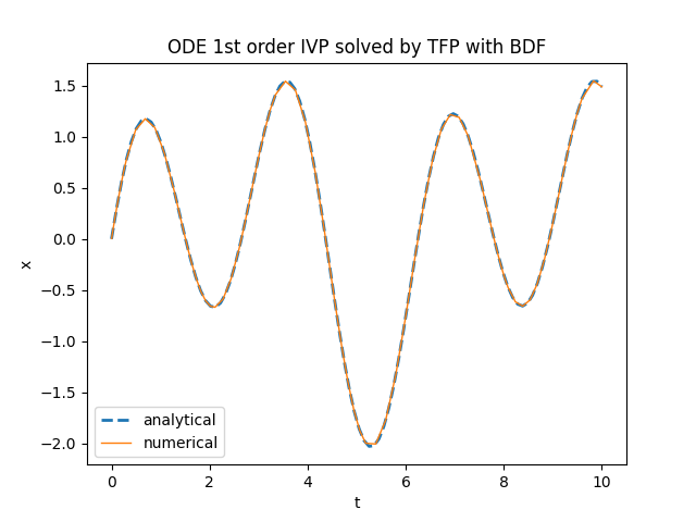
Comparison of the analytical solution with the numerical solution obtained by
.
tfp.math.ode.BDFTorchDiffEq
TorchDiffEq uses the torchdiffeq.odeint function
to numerically solve an ordinary first order differential equation of first order with initial value.
The explicit form of the above equation in Python with Torch is implemented as follows:
lambda t, x: torch.sin(t) + 3. * torch.cos(2. * t) - xBelow is an example of Python code that compares the analytical solution with the numerical one obtained by
torchdiffeq.odeint:
import numpy as np
import matplotlib.pyplot as plt

import torch
from torchdiffeq import odeint

ode_fn = lambda t, x: torch.sin(t) + 3. * torch.cos(2. * t) - x

an_sol = lambda t : (1./2.) * np.sin(t) - (1./2.) * np.cos(t) + \
                    (3./5.) * np.cos(2.*t) + (6./5.) * np.sin(2.*t) - \
                    (1./10.) * np.exp(-t)

t_begin=0.
t_end=10.
t_nsamples=100
t_space = np.linspace(t_begin, t_end, t_nsamples)
x_init = torch.tensor([0.])

x_an_sol = an_sol(t_space)

x_num_sol = odeint(ode_fn, x_init, torch.tensor(t_space))

plt.figure()
plt.plot(t_space, x_an_sol, '--', linewidth=2, label='analytical')
plt.plot(t_space, x_num_sol, linewidth=1, label='numerical')
plt.title('ODE 1st order IVP solved by TorchDiffEq')
plt.xlabel('t')
plt.ylabel('x')
plt.legend()
plt.show()

Comparison of the analytical solution with the numerical solution obtained by
torchdiffeq.odeint.TensorFlowDiffEq
TensorFlowDiffEq is a library that replicates with TensorFlow what TorchDiffEq achieves with Torch.
TensorFlowDiffEq uses the tfdiffeq.odeint function to numerically solve ordinary first order differential equations with initial value.
The explicit form of the above equation in Python with Tensorflow is implemented as follows:
lambda t, x: tf.math.sin(t) + 3. * tf.math.cos(2. * t) - xBelow is an example of Python code that compares the analytical solution with the numerical one obtained by
tfdiffeq.odeint:
import numpy as np
import matplotlib.pyplot as plt

import tensorflow as tf
from tfdiffeq import odeint

ode_fn = lambda t, x: tf.math.sin(t) + 3. * tf.math.cos(2. * t) - x

an_sol = lambda t : (1./2.) * np.sin(t) - (1./2.) * np.cos(t) + \
                    (3./5.) * np.cos(2.*t) + (6./5.) * np.sin(2.*t) - \
                    (1./10.) * np.exp(-t)

t_begin=0.
t_end=10.
t_nsamples=100
t_space = np.linspace(t_begin, t_end, t_nsamples)
x_init = tf.constant([0.])

x_an_sol = an_sol(t_space)

x_num_sol = odeint(ode_fn, x_init, tf.constant(t_space))

plt.figure()
plt.plot(t_space, x_an_sol, '--', linewidth=2, label='analytical')
plt.plot(t_space, x_num_sol, linewidth=1, label='numerical')
plt.title('ODE 1st order IVP solved by TensorFlowDiffEq')
plt.xlabel('t')
plt.ylabel('x')
plt.legend()
plt.show()
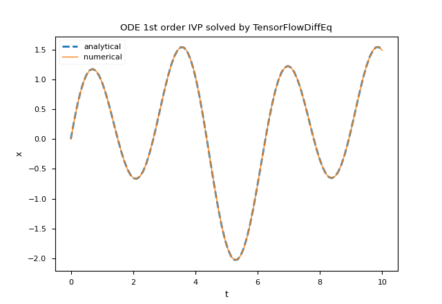
Comparison of the analytical solution with the numerical solution obtained by
tfdiffeq.odeint.NeuroDiffEq
NeuroDiffEq is a library that uses a neural network implemented via PyTorch
to numerically solve a first order differential equation with initial value.
The NeuroDiffEq solver has a number of differences from previous solvers. First of all the differential equation must be represented in implicit form:
$$ \begin{equation}
x'+x-\sin t - 3 \cos 2t = 0
\end{equation} $$
moreover the function diff(x, t, order) allows to indicate the first derivative and finally the lambda (or function) representing the equation has the $t$ and the $x$ inverted position.
For what just said the implicit form of the above equation in Python with Torch and NeuroDiffEq is implemented as follows:
lambda x, t: diff(x, t, order=1) + x - torch.sin(t) - 3. * torch.cos(2. * t)The library NeuroDiffEq uses the
neurodiffeq.ode.solve function to approximate the solution of the equation;
this function takes in input (optionally) a neural network, the training algorithm and other hyperparameters.Below is an example of Python code that compares the analytical solution with the numerical solution obtained by
neurodiffeq.ode.solve.
in the range $[0.0,2.0]$ with the following settings:
- Fully Connected neural network (abbreviated FC, also known as MLP for multilayer perceptron) with 6 layers, 50 neurons per layer and Tanh as activation function;
- SGD as optimization algorithm with learing rate set to 0.001;
- batch size set to 30, max number of epochs set to 1000, best model flag set to True.
import numpy as np
import matplotlib.pyplot as plt
import torch

from neurodiffeq import diff
from neurodiffeq.ode import solve
from neurodiffeq.ode import IVP
from neurodiffeq.ode import Monitor
import neurodiffeq.networks as ndenw

ode_fn = lambda x, t: diff(x, t, order=1) + x - torch.sin(t) - 3. * torch.cos(2. * t)

an_sol = lambda t : (1./2.) * np.sin(t) - (1./2.) * np.cos(t) + \
                    (3./5.) * np.cos(2.*t) + (6./5.) * np.sin(2.*t) - \
                    (1./10.) * np.exp(-t)

t_begin=0.
t_end=2.
t_nsamples=100
t_space = np.linspace(t_begin, t_end, t_nsamples)
x_init = IVP(t_0=t_begin, x_0=0.0)

x_an_sol = an_sol(t_space)

net = ndenw.FCNN(n_hidden_layers=6, n_hidden_units=50, actv=torch.nn.Tanh)
optimizer = torch.optim.SGD(net.parameters(), lr=0.001)
num_sol, loss_sol = solve(ode_fn, x_init, t_min=t_begin, t_max=t_end,
	batch_size=30,
	max_epochs=1000,
	return_best=True,
	net=net,
	optimizer=optimizer,
	monitor=Monitor(t_min=t_begin, t_max=t_end, check_every=10))
x_num_sol = num_sol(t_space, as_type='np')

plt.figure()
plt.plot(t_space, x_an_sol, '--', linewidth=2, label='analytical')
plt.plot(t_space, x_num_sol, linewidth=1, label='numerical')
plt.title('ODE 1st order IVP solved by NeuroDiffEq')
plt.xlabel('t')
plt.ylabel('x')
plt.legend()
plt.show()
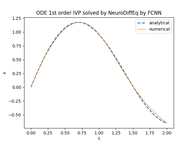
Comparison of the analytical solution with the numerical solution obtained by
neurodiffeq.ode.solve.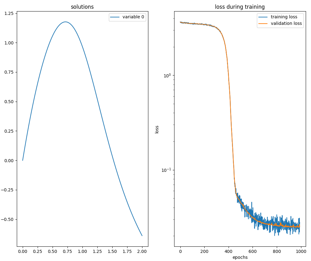
Graph of the monitor at the end of the training performed by
neurodiffeq.ode.solve.System of two ODEs of first order with IVP
Let the following system of two ordinary differential equations with initial values be given:
$$ \begin{equation}
\begin{cases}
x' + x − y = 0
\\
y' - 4x + y = 0
\\
x(0)=2
\\
y(0)=0
\end{cases}
\end{equation} $$
whose analytical solution is:
$$ \begin{equation}
\begin{cases}
x(t) = e^t + e^{-3 t}
\\
y(t) = 2 e^t - 2 e^{-3 t}
\end{cases}
\end{equation} $$
verifiable online via Wolfram Alpha.
Implementations of the following resolutions require the differential equations to be written explicitly in the forms $x'=F_1(x,y,t)$ and $y'=F_2(x,y,t)$
and then the two equations become:
$$ \begin{equation}
\begin{cases}
x' = y - x
\\
y' = 4x - y
\end{cases}
\end{equation} $$
and in matrix form:
$$\left[\begin{matrix} x' \\ y' \end{matrix} \right] = \left[\begin{matrix} -1 & 1 \\ 4 & -1 \end{matrix} \right] \left[\begin{matrix} x \\ y \end{matrix} \right] $$
Scipy
Scipy uses the scipy.integrate.solve_ivp function
to numerically solve a system of ordinary first order differential equations of first order with initial values.
The explicit form of the above pair of equations in Python with NumPy is implemented as follows:
def ode_sys(t, XY):
	x=XY[0]
	y=XY[1]
	dx_dt= - x + y
	dy_dt= 4. * x - y
	return [dx_dt, dy_dt]
Alternatively, the system represented in matrix form in Python with Scipy is implemented as follows:
A = [[-1., 1.],
    [4., -1.]]

ode_sys = lambda t, XY : A @ XY
Note that the second argument is an array of size two, which is as much as the number of unknown functions.
Below is an example of Python code that compares the analytical solution of the system with the numerical one obtained by
scipy.integrate.solve_ivp:
import numpy as np
import matplotlib.pyplot as plt

from scipy.integrate import solve_ivp

def ode_sys(t, XY):
	x=XY[0]
	y=XY[1]
	dx_dt= - x + y
	dy_dt= 4. * x - y
	return [dx_dt, dy_dt]

an_sol_x = lambda t : np.exp(t) + np.exp(-3. * t)
an_sol_y = lambda t : 2. * np.exp(t) - 2. * np.exp(-3. * t)

t_begin=0.
t_end=5.
t_nsamples=100
t_space = np.linspace(t_begin, t_end, t_nsamples)
x_init = 2.
y_init = 0.

x_an_sol = an_sol_x(t_space)
y_an_sol = an_sol_y(t_space)

method = 'RK45' #available methods: 'RK45', 'RK23', 'DOP853', 'Radau', 'BDF', 'LSODA'
num_sol = solve_ivp(ode_sys, [t_begin, t_end], [x_init, y_init], method=method, dense_output=True)
XY_num_sol = num_sol.sol(t_space)
x_num_sol = XY_num_sol[0].T
y_num_sol = XY_num_sol[1].T

plt.figure()
plt.plot(t_space, x_an_sol, '--', linewidth=2, label='analytical x')
plt.plot(t_space, y_an_sol, '--', linewidth=2, label='analytical y')
plt.plot(t_space, x_num_sol, linewidth=1, label='numerical x')
plt.plot(t_space, y_num_sol, linewidth=1, label='numerical y')
plt.title('System of 2 ODEs 1st order IVP solved by SciPy with method=' + method)
plt.xlabel('t')
plt.legend()
plt.show()
Here the link for the matrix form variation on GitHub.
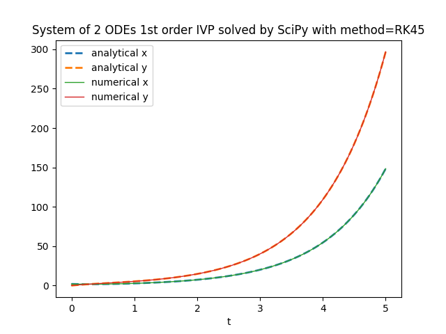
Comparison of the analytical solution of the system with the numerical solution obtained by
scipy.integrate.solve_ivp.TensorFlow Probability
TensorFlow Probability uses the tfp.math.ode.BDF class
to numerically solve a system of ordinary first order differential equations with initial values.
The explicit form of the above pair of equations in Python with TensorFlow Probability is implemented as follows:
def ode_sys(t, XY):
	x=XY[0]
	y=XY[1]
	dx_dt= - x + y
	dy_dt= 4. * x - y
	return [dx_dt, dy_dt]
Alternatively, the system represented in matrix form in Python with TensorFlow Probability is implemented as follows:
A = tf.constant([[-1., 1.], [4., -1.]])

ode_sys = lambda t, XY : tf.linalg.matvec(A, XY)
Note that the second argument is an array of size two, which is as much as the number of unknown functions.
Below is an example of Python code that compares the analytical solution with the numerical one obtained by
tfp.math.ode.BDF:
import numpy as np
import matplotlib.pyplot as plt

import tensorflow as tf
import tensorflow_probability as tfp

def ode_sys(t, XY):
	x=XY[0]
	y=XY[1]
	dx_dt= - x + y
	dy_dt= 4. * x - y
	return [dx_dt, dy_dt]

an_sol_x = lambda t : np.exp(t) + np.exp(-3. * t)
an_sol_y = lambda t : 2. * np.exp(t) - 2. * np.exp(-3. * t)

t_begin=0.
t_end=5.
t_nsamples=100
t_space = np.linspace(t_begin, t_end, t_nsamples)
t_init = tf.constant(t_begin)
x_init = tf.constant(2.)
y_init = tf.constant(0.)

x_an_sol = an_sol_x(t_space)
y_an_sol = an_sol_y(t_space)

num_sol = tfp.math.ode.BDF().solve(ode_sys, t_init, [x_init, y_init],
	solution_times=tfp.math.ode.ChosenBySolver(tf.constant(t_end)) )

plt.figure()
plt.plot(t_space, x_an_sol, '--', linewidth=2, label='analytical x')
plt.plot(t_space, y_an_sol, '--', linewidth=2, label='analytical y')
plt.plot(num_sol.times, num_sol.states[0], linewidth=1, label='numerical x')
plt.plot(num_sol.times, num_sol.states[1], linewidth=1, label='numerical y')
plt.title('System of two ODEs 1st order IVP solved by TFP with BDF')
plt.xlabel('t')
plt.legend()
plt.show()
Here the link for the matrix form variation on GitHub.
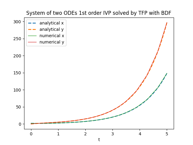
Comparison of the analytical solution of the system with the numerical solution obtained by
.
tfp.math.ode.BDFTorchDiffEq
TorchDiffEq uses the torchdiffeq.odeint function
to numerically solve a system of ordinary first order differential equations with initial values.
The explicit form of the above pair of equations in Python with Torch is implemented as follows:
def ode_sys(t, XY):
	x=XY[0]
	y=XY[1]
	dx_dt= torch.Tensor([- x + y])
	dy_dt= torch.Tensor([4. * x - y])
	return torch.cat([dx_dt, dy_dt])
Alternatively, the system represented in matrix form in Python with Torch is implemented as follows:
A = torch.Tensor([[-1., 1.],
                  [4., -1.]])

ode_sys = lambda t, XY : A @ XY
Note that the second argument is an array of size two, which is as much as the number of unknown functions.
Below is an example of Python code that compares the analytical solution with the numerical one obtained by
torchdiffeq.odeint:
import numpy as np
import matplotlib.pyplot as plt

import torch
from torchdiffeq import odeint

def ode_sys(t, XY):
	x=XY[0]
	y=XY[1]
	dx_dt= torch.Tensor([- x + y])
	dy_dt= torch.Tensor([4. * x - y])
	return torch.cat([dx_dt, dy_dt])

an_sol_x = lambda t : np.exp(t) + np.exp(-3. * t)
an_sol_y = lambda t : 2. * np.exp(t) - 2. * np.exp(-3. * t)

t_begin=0.
t_end=5.
t_nsamples=100
t_space = np.linspace(t_begin, t_end, t_nsamples)
x_init = torch.Tensor([2.])
y_init = torch.Tensor([0.])

x_an_sol = an_sol_x(t_space)
y_an_sol = an_sol_y(t_space)

num_sol = odeint(ode_sys, torch.cat([x_init, y_init]), torch.Tensor(t_space)).numpy()

plt.figure()
plt.plot(t_space, x_an_sol, '--', linewidth=2, label='analytical x')
plt.plot(t_space, y_an_sol, '--', linewidth=2, label='analytical y')
plt.plot(t_space, num_sol[:,0], linewidth=1, label='numerical x')
plt.plot(t_space, num_sol[:,1], linewidth=1, label='numerical y')
plt.title('System of two ODEs 1st order IVP solved by TorchDiffEq')
plt.xlabel('t')
plt.legend()
plt.show()
Here the link for the matrix form variation on GitHub.
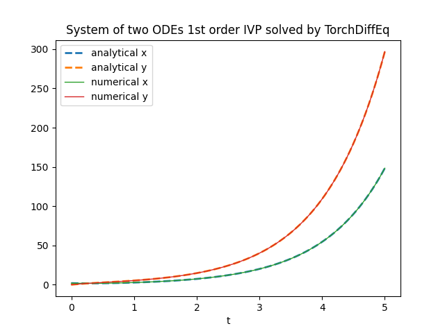
Comparison of the analytical solution os the system with the numerical solution obtained by
torchdiffeq.odeint.TensorFlowDiffEq
TensorFlowDiffEq uses the tfdiffeq.odeint function
to numerically solve a system of ordinary first order differential equations with initial values.
The explicit form of the above pair of equations in Python with TensorFlow is implemented as follows:
def ode_sys(t, XY):
	x=XY[0]
	y=XY[1]
	dx_dt= - x + y
	dy_dt= 4. * x - y
	return tf.stack([dx_dt, dy_dt])
Alternatively, the system represented in matrix form in Python with TensorFlow is implemented as follows:
A = tf.constant([[-1., 1.],
                 [4., -1.]],
                 dtype=tf.float64)

ode_sys = lambda t, XY : A @ XY
Note that the second argument is an array of size two, which is as much as the number of unknown functions.
Below is an example of Python code that compares the analytical solution with the numerical one obtained by
tfdiffeq.odeint:
import numpy as np
import matplotlib.pyplot as plt

import tensorflow as tf
from tfdiffeq import odeint

def ode_sys(t, XY):
	x=XY[0]
	y=XY[1]
	dx_dt= - x + y
	dy_dt= 4. * x - y
	return tf.stack([dx_dt, dy_dt])

an_sol_x = lambda t : np.exp(t) + np.exp(-3. * t)
an_sol_y = lambda t : 2. * np.exp(t) - 2. * np.exp(-3. * t)

t_begin=0.
t_end=5.
t_nsamples=100
t_space = np.linspace(t_begin, t_end, t_nsamples)
x_init = tf.constant([2.])
y_init = tf.constant([0.])

x_an_sol = an_sol_x(t_space)
y_an_sol = an_sol_y(t_space)

num_sol = odeint(
    ode_sys,
    tf.convert_to_tensor([x_init, y_init], dtype=tf.float64),
    tf.constant(t_space)).numpy()

plt.figure()
plt.plot(t_space, x_an_sol, '--', linewidth=2, label='analytical x')
plt.plot(t_space, y_an_sol, '--', linewidth=2, label='analytical y')
plt.plot(t_space, num_sol[:,0], linewidth=1, label='numerical x')
plt.plot(t_space, num_sol[:,1], linewidth=1, label='numerical y')
plt.title('System of two ODEs 1st order IVP solved by TensorFlowDiffEq')
plt.xlabel('t')
plt.legend()
plt.show()
Here the link for the matrix form variation on GitHub.
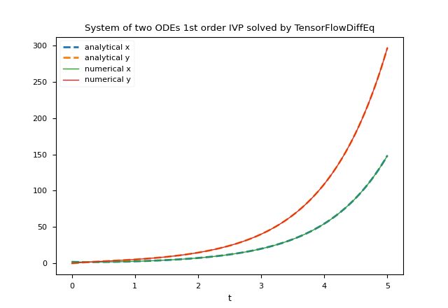
Comparison of the analytical solution os the system with the numerical solution obtained by
tfdiffeq.odeint.NeuroDiffEq
NeuroDiffEq is a library that uses a neural network implemented via PyTorch
to numerically solve a system of differential equations with initial values.
As said above, the NeuroDiffEq solver has a number of differences from previous solvers. First of all the system of differential equations must be represented in implicit form:
$$ \begin{equation}
\begin{cases}
x' + x − y = 0
\\
y' - 4x + y = 0
\end{cases}
\end{equation} $$
moreover the function diff(x, t, order) allows to indicate the first derivative of $x$ with respect to $t$ and diff(x, t, order) the first derivative of $y$ with respect to $t$.
Finally, the lambda (or function) that represents the system takes as input three parameters in the order $x$, $y$ and $t$ respectively and returns an array
with size equal to the number of equations (in this case two-dimensional) to return the value of the left-hand expressions of the equations.
For what just said the implicit form of the above system in Python with Torch and NeuroDiffEq is implemented as follows:
lambda x, y, t: [diff(x, t, order=1) + x - y, diff(y, t, order=1) - 4. * x + y ]The library NeuroDiffEq uses the
neurodiffeq.ode.solve_system function to approximate the solution of the system;
this function takes in input (optionally) a neural network, the training algorithm and other hyperparameters.Below is an example of Python code that compares the analytical solution with the numerical solution obtained by
neurodiffeq.ode.solve_system.
in the range $[0.0,2.0]$ with the following settings:
- Fully Connected neural network (abbreviated FC, also known as MLP for multilayer perceptron) with 3 layers, 50 neurons per layer and SinActv as activation function;
- Adam as optimization algorithm with learing rate set to 0.003;
- batch size set to 200, max number of epochs set to 1200, best model flag set to True.
import numpy as np
import matplotlib.pyplot as plt
import torch

from neurodiffeq import diff
from neurodiffeq.ode import solve_system
from neurodiffeq.ode import IVP
from neurodiffeq.ode import Monitor
import neurodiffeq.networks as ndenw

ode_sys = lambda x, y, t: [diff(x, t, order=1) + x - y, diff(y, t, order=1) - 4. * x + y ]

an_sol_x = lambda t : np.exp(t) + np.exp(-3. * t)
an_sol_y = lambda t : 2. * np.exp(t) - 2. * np.exp(-3. * t)

t_begin=0.
t_end=2.
t_nsamples=100
t_space = np.linspace(t_begin, t_end, t_nsamples)
x_init = IVP(t_0=t_begin, x_0=2.0)
y_init = IVP(t_0=t_begin, x_0=0.0)

x_an_sol = an_sol_x(t_space)
y_an_sol = an_sol_y(t_space)

batch_size=200

net = ndenw.FCNN(
	n_input_units=1,
        n_output_units=2,
	n_hidden_layers=3,
	n_hidden_units=50,
	actv=ndenw.SinActv)

optimizer = torch.optim.Adam(net.parameters(), lr=0.003)

num_sol, history = solve_system(
	ode_system=ode_sys,
	conditions=[x_init, y_init],
	t_min=t_begin,
	t_max=t_end,
	batch_size=batch_size,
	max_epochs=1200,
	return_best=True,
	single_net = net,
	optimizer=optimizer,
	monitor=Monitor(t_min=t_begin, t_max=t_end, check_every=10))
num_sol = num_sol(t_space, as_type='np')

plt.figure()
plt.plot(t_space, x_an_sol, '--', linewidth=2, label='analytical x')
plt.plot(t_space, y_an_sol, '--', linewidth=2, label='analytical y')
plt.plot(t_space, num_sol[0], linewidth=1, label='numerical x')
plt.plot(t_space, num_sol[1], linewidth=1, label='numerical y')
plt.title('System of two ODEs 1st order IVP solved by NeuroDiffEq')
plt.xlabel('t')
plt.legend()
plt.show()
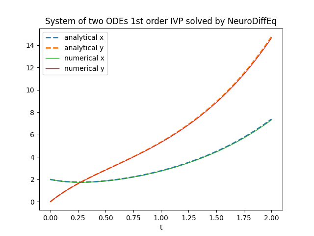
Comparison of the analytical solution with the numerical solution obtained by
neurodiffeq.ode.solve_system.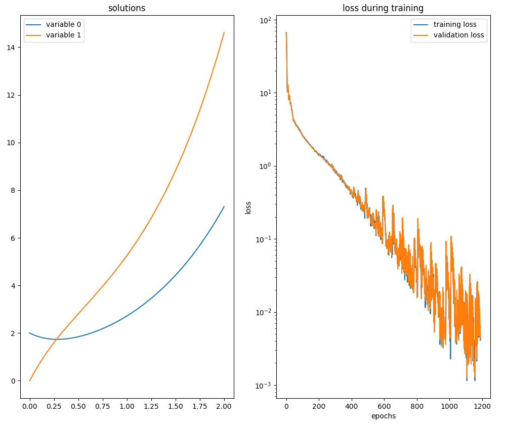
Graph of the monitor at the end of the training performed by
neurodiffeq.ode.solve_system.Second order ODE with IVP
Let the following Cauchy problem be given:
$$ \begin{equation}
\begin{cases}
x'' + x' + 2x = 0
\\
x(0)=1
\\
x'(0)=0
\end{cases}
\end{equation} $$
whose analytical solution is:
$$ x(t) = e^{\frac{-t}{2}} (\cos {\sqrt{7} \frac{t}{2}} + \frac{\sin {\sqrt{7} \frac{t}{2}}}{\sqrt{7}}) $$
verifiable online via Wolfram Alpha.
Implementations of the following resolutions require the differential equation of second order
to be written explicitly in the form as a system of two equations of first order as follows:
$$ \begin{equation}
\begin{cases}
y=x'
\\
y'=F(x, y, t)
\end{cases}
\end{equation} $$
and then the initial Cauchy problem is written equivalently in the following way:
$$ \begin{equation}
\begin{cases}
y = x'
\\
y'= -y - 2x = 0
\\
x(0)=1
\\
y(0)=0
\end{cases}
\end{equation} $$
Scipy
Scipy uses the scipy.integrate.solve_ivp function
to numerically solve a system of ordinary first order differential equations with initial values,
that, because of what was said before, is equivalent to the second-order equation with the same initial conditions.
The explicit form of the above system in Python with NumPy is implemented as follows:
def ode_sys(t, X):
        x=X[0]
        dx_dt=X[1]
        d2x_dt2=-dx_dt - 2*x
        return [dx_dt, d2x_dt2]
Below is an example of Python code that compares the analytical solution with the numerical one obtained by
scipy.integrate.solve_ivp:
import numpy as np
import matplotlib.pyplot as plt

from scipy.integrate import solve_ivp

def ode_sys(t, X):
	x=X[0]
	dx_dt=X[1]
	d2x_dt2=-dx_dt - 2*x
	return [dx_dt, d2x_dt2]

an_sol_x = lambda t : \
	np.exp(-t/2.) * (np.cos(np.sqrt(7) * t / 2.) + \
	np.sin(np.sqrt(7) * t / 2.)/np.sqrt(7.))

t_begin=0.
t_end=12.
t_nsamples=100
t_space = np.linspace(t_begin, t_end, t_nsamples)
x_init = 1.
dxdt_init = 0.

x_an_sol = an_sol_x(t_space)

method = 'RK45' #available methods: 'RK45', 'RK23', 'DOP853', 'Radau', 'BDF', 'LSODA'
num_sol = solve_ivp(ode_sys, [t_begin, t_end], [x_init, dxdt_init], method=method, dense_output=True)
X_num_sol = num_sol.sol(t_space)
x_num_sol = X_num_sol[0].T

plt.figure()
plt.plot(t_space, x_an_sol, '--', linewidth=2, label='analytical')
plt.plot(t_space, x_num_sol, linewidth=1, label='numerical')
plt.title('ODE 2nd order IVP solved by SciPy with method=' + method)
plt.xlabel('t')
plt.ylabel('x')
plt.legend()
plt.show()
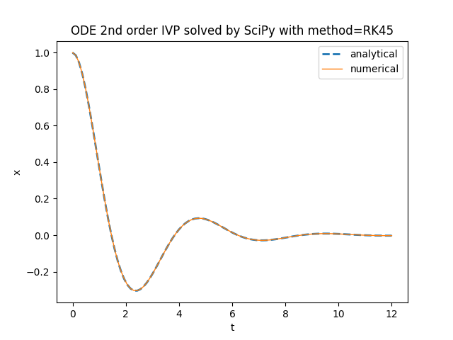
Comparison of the analytical solution of the second order equation with the numerical solution obtained by
scipy.integrate.solve_ivp.TensorFlow Probability
TensorFlow Probability uses the tfp.math.ode.BDF class
to numerically solve a system of ordinary first order differential equations with initial values,
that, because of what was said before, is equivalent to the second-order equation with the same initial conditions.
The explicit form of the above system in Python with TensorFlow Probability is implemented as follows:
def ode_sys(t, X):
	x=X[0]
	dx_dt=X[1]
	d2x_dt2=-dx_dt - 2*x
	return [dx_dt, d2x_dt2]
Below is an example of Python code that compares the analytical solution with the numerical one obtained by
tfp.math.ode.BDF:
import numpy as np
import matplotlib.pyplot as plt

import tensorflow as tf
import tensorflow_probability as tfp

def ode_sys(t, X):
	x=X[0]
	dx_dt=X[1]
	d2x_dt2=-dx_dt - 2*x
	return [dx_dt, d2x_dt2]

an_sol_x = lambda t : \
	np.exp(-t/2.) * (np.cos(np.sqrt(7) * t / 2.) + \
	np.sin(np.sqrt(7) * t / 2.)/np.sqrt(7.))

t_begin=0.
t_end=12.
t_nsamples=100
t_space = np.linspace(t_begin, t_end, t_nsamples)
t_init = tf.constant(t_begin)
x_init = tf.constant(1.)
dxdt_init = tf.constant(0.)

x_an_sol = an_sol_x(t_space)

num_sol = tfp.math.ode.BDF().solve(ode_sys, t_init, [x_init, dxdt_init],
	solution_times=tfp.math.ode.ChosenBySolver(tf.constant(t_end)) )

plt.figure()
plt.plot(t_space, x_an_sol, '--', linewidth=2, label='analytical')
plt.plot(num_sol.times, num_sol.states[0], linewidth=1, label='numerical')
plt.title('ODE 2nd order IVP solved by TFP with BDF')
plt.xlabel('t')
plt.ylabel('x')
plt.legend()
plt.show()
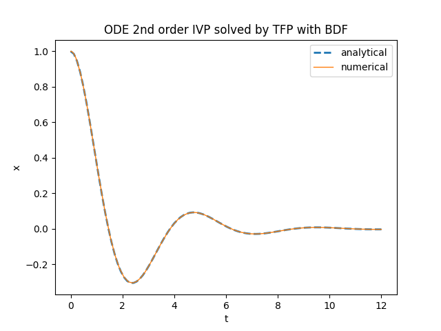
Comparison of the analytical solution of the second order equation with the numerical solution obtained by
.
tfp.math.ode.BDFTorchDiffEq
TorchDiffEq uses the torchdiffeq.odeint function
to numerically solve a system of ordinary first order differential equations with initial values,
that, because of what was said before, is equivalent to the second-order equation with the same initial conditions.
The explicit form of the above system in Python with Torch is implemented as follows:
def ode_sys(t, X):
	x=torch.Tensor([X[0]])
	dx_dt=torch.Tensor([X[1]])
	d2x_dt2=torch.Tensor([-dx_dt - 2*x])
	return torch.cat([dx_dt, d2x_dt2])
Below is an example of Python code that compares the analytical solution with the numerical one obtained by
torchdiffeq.odeint:
import numpy as np
import matplotlib.pyplot as plt

import torch
from torchdiffeq import odeint

def ode_sys(t, X):
	x=torch.Tensor([X[0]])
	dx_dt=torch.Tensor([X[1]])
	d2x_dt2=torch.Tensor([-dx_dt - 2*x])
	return torch.cat([dx_dt, d2x_dt2])

an_sol_x = lambda t : \
	np.exp(-t/2.) * (np.cos(np.sqrt(7) * t / 2.) + \
	np.sin(np.sqrt(7) * t / 2.)/np.sqrt(7.))

t_begin=0.
t_end=12.
t_nsamples=100
t_space = np.linspace(t_begin, t_end, t_nsamples)
x_init = torch.Tensor([1.])
dxdt_init = torch.Tensor([0.])

x_an_sol = an_sol_x(t_space)

num_sol = odeint(ode_sys, torch.cat([x_init, dxdt_init]), torch.Tensor(t_space)).numpy()

plt.figure()
plt.plot(t_space, x_an_sol, '--', linewidth=2, label='analytical')
plt.plot(t_space, num_sol[:,0], linewidth=1, label='numerical')
plt.title('ODE 2nd order IVP solved by TorchDiffEq')
plt.xlabel('t')
plt.ylabel('x')
plt.legend()
plt.show()
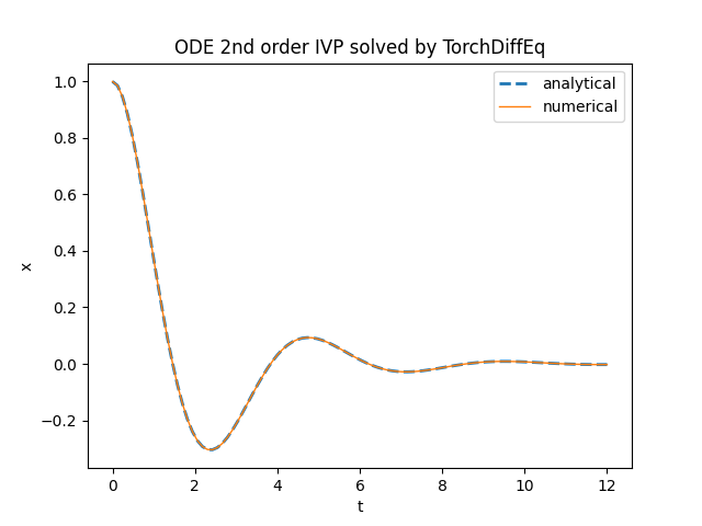
Comparison of the analytical solution of the second order equation with the numerical solution obtained by
torchdiffeq.odeint.TensorFlowDiffEq
TensorFlowDiffEq uses the tfdiffeq.odeint function
to numerically solve a system of ordinary differential equations of first order with initial values,
that, because of what was said before, is equivalent to the second-order equation with the same initial conditions.
The explicit form of the above system in Python with Tensorflow is implemented as follows:
def ode_sys(t, X):
	x=X[0]
	dx_dt=X[1]
	d2x_dt2=-dx_dt - 2*x
	return tf.stack([dx_dt, d2x_dt2])
Below is an example of Python code that compares the analytical solution with the numerical one obtained by
tfdiffeq.odeint:
import numpy as np
import matplotlib.pyplot as plt

import tensorflow as tf
from tfdiffeq import odeint

def ode_sys(t, X):
	x=X[0]
	dx_dt=X[1]
	d2x_dt2=-dx_dt - 2*x
	return tf.stack([dx_dt, d2x_dt2])

an_sol_x = lambda t : \
	np.exp(-t/2.) * (np.cos(np.sqrt(7) * t / 2.) + \
	np.sin(np.sqrt(7) * t / 2.)/np.sqrt(7.))

t_begin=0.
t_end=12.
t_nsamples=100
t_space = np.linspace(t_begin, t_end, t_nsamples)
x_init = tf.constant([1.])
dxdt_init = tf.constant([0.])

x_an_sol = an_sol_x(t_space)

num_sol = odeint(
	ode_sys,
	tf.convert_to_tensor([x_init, dxdt_init], dtype=tf.float64),
	tf.constant(t_space)).numpy()

plt.figure()
plt.plot(t_space, x_an_sol,'--', linewidth=2, label='analytical')
plt.plot(t_space, num_sol[:,0], linewidth=1, label='numerical')
plt.title('ODE 2nd order IVP solved by TensorFlowDiffEq')
plt.xlabel('t')
plt.ylabel('x')
plt.legend()
plt.show()
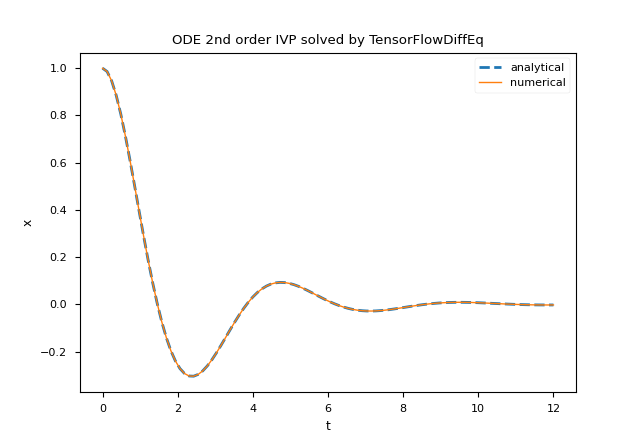
Comparison of the analytical solution of the second order with the numerical solution obtained by
tfdiffeq.odeint.NeuroDiffEq
NeuroDiffEq is a library that uses a neural network implemented via PyTorch
to numerically solve a second-order differential equation with initial values.
The NeuroDiffEq solver has a number of differences from previous solvers.
First of all, it is not necessary to rewrite the second-order equation in an equivalent first order system of equations
because the library natively supports derivatives of order higher than one,
in fact the function diff(x, t, order) allows you to indicate the first derivative passing order=1 and the second derivative passing order=2.
Because of the above, this library takes as input the equation in an implicit form, namely:
$$ \begin{equation}
x'' + x' + 2x = 0
\end{equation} $$
and keeping in mind that the lambda (or function) representing the equation has $t$ and $x$ inverted in position with respect to all other libraries seen before,
the implicit form of the above equation in Python with Torch and NeuroDiffEq is implemented like this:
ode_fn = lambda x, t: diff(x, t, order=2) + diff(x, t, order=1) + 2. * xThe library NeuroDiffEq uses the
neurodiffeq.ode.solve function to approximate the solution of the equation;
this function takes in input (optionally) a neural network, the training algorithm and other hyperparameters.Below is an example of Python code that compares the analytical solution with the numerical solution obtained by
neurodiffeq.ode.solve.
in the range $[0.0,12.0]$ with the following settings:
- Fully Connected neural network (abbreviated FC, also known as MLP for multilayer perceptron) with 6 layers, 50 neurons per layer and Tanh as activation function;
- Adam as optimization algorithm with learing rate set to 0.002;
- batch size set to 200, max number of epochs set to 500, best model flag set to True.
import numpy as np
import matplotlib.pyplot as plt
import torch

from neurodiffeq import diff
from neurodiffeq.ode import solve
from neurodiffeq.ode import IVP
from neurodiffeq.ode import Monitor
import neurodiffeq.networks as ndenw

ode_fn = lambda x, t: diff(x, t, order=1) + x - torch.sin(t) - 3. * torch.cos(2. * t)

an_sol = lambda t : (1./2.) * np.sin(t) - (1./2.) * np.cos(t) + \
                    (3./5.) * np.cos(2.*t) + (6./5.) * np.sin(2.*t) - \
                    (1./10.) * np.exp(-t)

t_begin=0.
t_end=2.
t_nsamples=100
t_space = np.linspace(t_begin, t_end, t_nsamples)
x_init = IVP(t_0=t_begin, x_0=0.0)

x_an_sol = an_sol(t_space)

net = ndenw.FCNN(n_hidden_layers=6, n_hidden_units=50, actv=torch.nn.Tanh)
optimizer = torch.optim.SGD(net.parameters(), lr=0.001)
num_sol, loss_sol = solve(ode_fn, x_init, t_min=t_begin, t_max=t_end,
	batch_size=30,
	max_epochs=1000,
	return_best=True,
	net=net,
	optimizer=optimizer,
	monitor=Monitor(t_min=t_begin, t_max=t_end, check_every=10))
x_num_sol = num_sol(t_space, as_type='np')

plt.figure()
plt.plot(t_space, x_an_sol, '--', linewidth=2, label='analytical')
plt.plot(t_space, x_num_sol, linewidth=1, label='numerical')
plt.title('ODE 1st order IVP solved by NeuroDiffEq')
plt.xlabel('t')
plt.ylabel('x')
plt.legend()
plt.show()
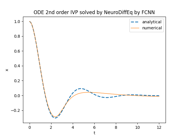
Comparison of the analytical solution of the second order with the numerical solution obtained by
neurodiffeq.ode.solve.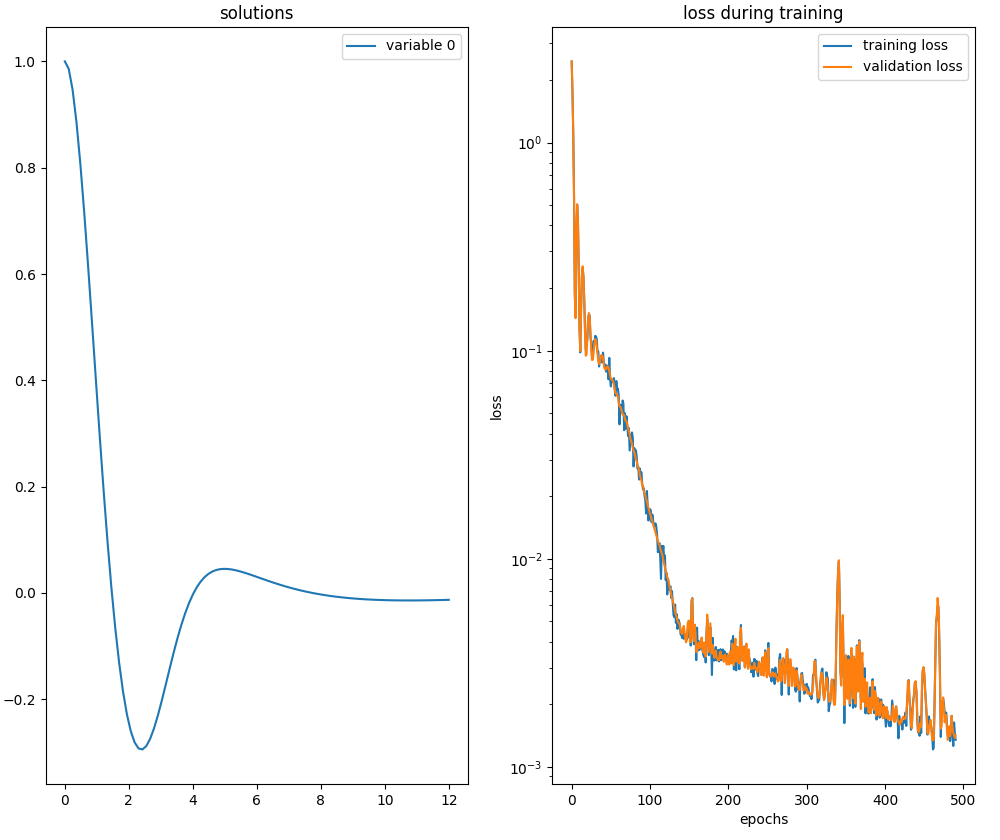
Graph of the monitor at the end of the training performed by
neurodiffeq.ode.solve.Download of the complete code
The complete code is available at GitHub.
These materials are distributed under MIT license; feel free to use, share, fork and adapt these materials as you see fit.
Also please feel free to submit pull-requests and bug-reports to this GitHub repository or contact me on my social media channels available on the top right corner of this page.