Experiments with Neural ODEs in Julia
Neural Ordinary Differential Equations (abbreviated Neural ODEs) is a paper that introduces a new family of neural networks
in which some hidden layers (or even the only layer in the simplest cases) are implemented with an ordinary differential equation solver.
This post shows three examples written in Julia (there will be more in the future) that use some of the ideas described in the Neural ODEs paper to show possible solutions in the following scenarios:
- Experiment #1: train a system of ODEs to meet an objective.
- Experiment #2: calculate the forecast of a time series system described by a differential law.
- Experiment #3: fit a function with MLP and Neural ODEs
To get the code see paragraph Download the complete code at the end of this post.
Conventions
In this post the conventions used are as follows:
- $t$ is the independent variable
- $x$ is the unknown function
- $y$ is the second unknown function
- $x$ and $y$ are intended to be functions of $t$, so $x=x(t)$ and $y=y(t)$, but the use of this compact notation, in addition to having a greater readability at a mathematical level makes it easier to "translate" the equation into code
- $x'$ is the first derivative of x with respect to $t$ and of course $y'$ is the first derivative of y with respect to $t$
Experiment #1: train a system of ODEs to meet an objective
A multilayer perceptron (abbreviated MLP) is an appropriate tool for learning a nonlinear relationship between inputs and outputs whose law is not known.
On the other hand, there are cases where one has a priori knowledge of the law that correlates inputs and outputs, for example in the form of a parametric system of differential equations:
in this situation a neural network of type MLP does not allow to use such knowledge while a network of type Neural ODEs does.
The application scenario
The application scenario is as follows:
- A dataset that contains the inputs and outputs
- A law that associates input and output in the form of a parametric system of differential equations
- Determine appropriate parameter values so that the system obtained by replacing the formal parameters with the determined values best approximates the mapping between input and output.
In this post, the law is intentionally not a famous law, but is the parametric system of two first-order equations and eight parameters shown in the following paragraph.
The problem to be solved
Let the following parametric system of two ordinary differential equations with initial values be given
which represents the law describing the behavior of a hypothetical dynamical system:
$$ \begin{equation}
\begin{cases}
x' = a_1x + b_1y + c_1e^{-d_1t}
\\
y'= a_2x + b_2y + c_2e^{-d_2t}
\\
x(0)=0
\\
y(0)=0
\end{cases}
\end{equation} $$
Obviously this is a demo whose purpose is to test the goodness of the method, so to prepare the dataset
we arbitrarily set eight parameter values, for example these:
$$ \left[\begin{matrix}a_1 \\ b_1 \\ c_1 \\ d_1 \\ a_2 \\ b_2 \\ c_2 \\ d_2 \end{matrix} \right] =
\left[\begin{matrix}1.11 \\ 2.43 \\ -3.66 \\ 1.37 \\ 2.89 \\ -1.97 \\ 4.58 \\ 2.86 \end{matrix} \right] $$
and knowing that with such parameter values the analytical solution is as follows:
$$ \begin{equation}
\begin{array}{l}
x(t) = \\
\;\; -1.38778 \cdot 10^{-17} \; e^{-8.99002 t} - \\
\;\; 2.77556 \cdot 10^{-17} \; e^{-7.50002 t} + \\
\;\; 3.28757 \; e^{-3.49501 t} - \\
\;\; 3.18949 \; e^{-2.86 t} + \\
\;\; 0.258028 \; e^{-1.37 t} - \\
\;\; 0.356108 \; e^{2.63501 t} + \\
\;\; 4.44089 \cdot 10^{-16} \; e^{3.27002 t} + \\
\;\; 1.11022 \cdot 10^{-16} \; e^{4.76002 t} \\
\\
y(t) = \\
\;\; -6.23016 \; e^{-3.49501 t} + \\
\;\; 5.21081 \; e^{-2.86 t} + \\
\;\; 1.24284 \; e^{-1.37 t} - \\
\;\; 0.223485 \; e^{2.63501 t} + \\
\;\; 2.77556 \cdot 10^{-17} \; e^{4.76002 t} \\
\end{array}
\end{equation} $$
(verifiable online via Wolfram Alpha)
you are able to prepare the dataset: the input is a discretized interval of time from $0$ to $1.5$ step $0.01$,
while the output consists of the analytical solutions $x=x(t)$ and $y=y(t)$ for each $t$ belonging to the input.
Once the dataset is prepared, we forget about the values of the parameters and the analytical solution and we pose the problem
of how to train a neural network to determine an appropriate set of values for the eight parameters in order to best approximate
the non-linear mapping between input and output of the dataset.
Solution implementation
The parametric system of differential equations is already written in explicit form, and in Julia with DifferentialEquations it is implemented like this:
function parametric_ode_system!(du,u,p,t)
  x, y = u
  a1, b1, c1, d1, a2, b2, c2, d2 = p
  du[1] = dx = a1*x + b1*y + c1*exp(-d1*t)
  du[2] = dy = a2*x + b2*y + c2*exp(-d2*t)
end- Input: $t \in [0, 1.5]$ discretization step $0.01$
- Boundary conditions: $x(0)=0; y(0)=0$
- Initial values of any parameters; for convenience we set them all equal to $1$.
tbegin=0.0
tend=1.5
tstep=0.01
trange = tbegin:tstep:tend
u0 = [0.0,0.0]
tspan = (tbegin,tend)
p = ones(8)prob = ODEProblem(parametric_ode_system!, u0, tspan, p)
function net()
solve(prob, Tsit5(), p=p, saveat=trange)
endThe training settings are:
- Optimizator: ADAM
- Learning rate: $0.05$
- Number of epochs: $1000$
- Loss function: sum of squares of differences
epochs = 1000
learning_rate = 0.05
data = Iterators.repeated((), epochs)
opt = ADAM(learning_rate)
callback_func = function ()
#.......
end
fparams = Flux.params(p)
Flux.train!(loss_func, fparams, data, opt, cb=callback_func)Here is the complete code:
using Flux, DiffEqFlux, DifferentialEquations, Plots
function parametric_ode_system!(du,u,p,t)
x, y = u
a1, b1, c1, d1, a2, b2, c2, d2 = p
du[1] = dx = a1*x + b1*y + c1*exp(-d1*t)
du[2] = dy = a2*x + b2*y + c2*exp(-d2*t)
end
true_params = [1.11, 2.43, -3.66, 1.37, 2.89, -1.97, 4.58, 2.86]
an_sol_x(t) =
-1.38778e-17 * exp(-8.99002 * t) -
2.77556e-17 * exp(-7.50002 * t) +
3.28757 * exp(-3.49501 * t) -
3.18949 * exp(-2.86 * t) +
0.258028 * exp(-1.37 * t) -
0.356108 * exp(2.63501 * t) +
4.44089e-16 * exp(3.27002 * t) +
1.11022e-16 * exp(4.76002 * t)
an_sol_y(t) =
-6.23016 * exp(-3.49501 * t) +
5.21081 * exp(-2.86 * t) +
1.24284 * exp(-1.37 * t) -
0.223485 * exp(2.63501 * t) +
2.77556e-17 * exp(4.76002 * t)
tbegin=0.0
tend=1.5
tstep=0.01
trange = tbegin:tstep:tend
u0 = [0.0,0.0]
tspan = (tbegin,tend)
p = ones(8)
prob = ODEProblem(parametric_ode_system!, u0, tspan, p)

function net()
    solve(prob, Tsit5(), p=p, saveat=trange)
end
dataset_outs = [an_sol_x.(trange), an_sol_y.(trange)]
function loss_func()
pred = net()
sum(abs2, dataset_outs[1] .- pred[1,:]) +
sum(abs2, dataset_outs[2] .- pred[2,:])
end
epochs = 1000
learning_rate = 0.05
data = Iterators.repeated((), epochs)
opt = ADAM(learning_rate)
callback_func = function ()
println("loss: ", loss_func())
end
fparams = Flux.params(p)
Flux.train!(loss_func, fparams, data, opt, cb=callback_func)
predict_prob = ODEProblem(parametric_ode_system!, u0, tspan, p)
predict_sol = solve(prob, Tsit5(), saveat=trange)
x_predict_sol = [u[1] for u in predict_sol.u]
y_predict_sol = [u[2] for u in predict_sol.u]
println("Learned parameters:", p)
plot(trange, dataset_outs[1],
linewidth=2, ls=:dash,
title="Neural ODEs to fit params",
xaxis="t",
label="dataset x(t)",
legend=true)
plot!(trange, dataset_outs[2],
linewidth=2, ls=:dash,
label="dataset y(t)")
plot!(predict_sol.t, x_predict_sol,
linewidth=1,
label="predicted x(t)")
plot!(predict_sol.t, y_predict_sol,
linewidth=1,
label="predicted y(t)")
The parameter values obtained at the end of the training are as follows: $$ \left[\begin{matrix}a_1 \\ b_1 \\ c_1 \\ d_1 \\ a_2 \\ b_2 \\ c_2 \\ d_2 \end{matrix} \right] = \left[\begin{matrix}1.7302980833638142 \\ 1.2823312512074032 \\ -1.6866178290795755 \\ 0.41974163099782325 \\ 1.223075467559363 \\ 0.9410722500584323 \\ 0.18890958911958686 \\ 1.7462909509457183 \end{matrix} \right] $$ which are obviously different from the values of the parameters used to generate the dataset (passing through the analytical solution); but the system of equations obtained by replacing the formal parameters with these values obtained from the training of the neural network and solving numerically this last system we obtain a numerical solution that approximates quite well the dataset, as shown in the figure:
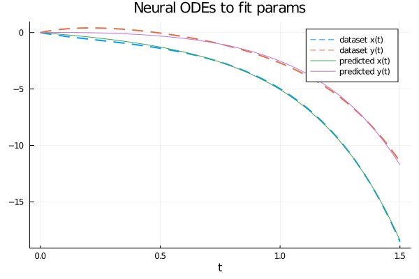
Ccomparison of the numerical solution that approximates the dataset.
Different training strategies allow to obtain different values of the parameters and therefore a different numerical solution of the system with a different accuracy.
Esperimento #2: calculate the forecast of a time series system described by a differential law
There are various taxonomies of black-box neural networks to compute the forecast of time series (see the post Forecast of a univariate equally spaced time series with TensorFlow on this website)
which are suitable when you do not have a priori knowledge of the mathematical law that describes the behavior of the input time series.
When instead we have a priori knowledge of the differential law that governs the evolution of the derivatives of time series
(for example in the form of a parametric system of differential equations)
a network of Neural ODE type becomes the right tool to calculate the forecast in an efficient and accurate way.
The application scenario
The application scenario is as follows:
- A dataset containing a set of interdependent time series.
- A law governing the evolution of time series derivatives over time in the form of a parametric system of differential equations.
The goal is twofold:
- 1. Train a NeuralODE type neural network to learn the value of ODE system parameters from the input time series.
- 2. Use the learned system to compute the forecast, then the predictions with time later than the initial time series.
In this post the law is different and is a law of oscillation with damping plus the forecast objective is addressed.
The problem to be solved
Let the following parametric system of two ordinary differential equations with initial values be given
representing the law describing the evolution of the derivatives of a pair of interdependent time series:
$$ \begin{equation}
\begin{cases}
\left[\begin{matrix}
x' & y'
\end{matrix} \right]
=
\left[\begin{matrix}
\sin 2x + \cos 2y \\ \sin 2x + \cos 2y
\end{matrix} \right] ^ \dag
\left[\begin{matrix}a_{11} & a_{12} \\ a_{21} & a_{22} \end{matrix} \right]
\\
x(0)=x_0
\\
y(0)=y_0
\end{cases}
\end{equation} $$
Obviously this is a demo whose purpose is to test the goodness of the method, so to prepare the dataset
let's set arbitrarily the values of the four parameters and the two initial conditions:
$$ A = \left[\begin{matrix}a_{11} & a_{12} \\ a_{21} & a_{22} \end{matrix} \right] =
\left[\begin{matrix}-0.15 & 2.10 \\ -2.10 & -0.10 \end{matrix} \right] $$
$$ \begin{equation}
\begin{cases}
x(0)=2.5
\\
y(0)=0.5
\end{cases}
\end{equation} $$
so that we can create the dataset of the true time series pair:
time is discretized arbitrarily from $0$ to $4$ with a number of $51$ discrete values,
while the time series $x(t)$ and $y(t)$ are constructed by solving the system of differential equations
obtained using the matrix A of the specific parameters in the parametric system above, along with arbitrarily chosen initial conditions.
Once the dataset is prepared (which in the real world can be obtained by performing real measurements)
we forget about the values of the parameters (which will then become unknown) and we have a twofold problem:
- how to train a neural network that incorporates the known law to learn the system at unknown parameters in order to best approximate the initial time series?
- how to use such neural net once trained to predict future values (the forecast, in fact)?
Solution implementation
The mathematical law of the system above in Julia is implemented as follows:
math_law(u) = sin.(2. * u) + cos.(2. * u)function true_ode(du,u,p,t)
true_A = [-0.15 2.10; -2.10 -0.10]
du .= ((math_law(u))'true_A)'
end
tbegin = 0.0
tend = 4.0
datasize = 51
t = range(tbegin,tend,length=datasize)
u0 = [2.5; 0.5]
tspan = (tbegin,tend)
trange = range(tbegin,tend,length=datasize)
prob = ODEProblem(true_ode, u0, tspan)
dataset_ts = Array(solve(prob, Tsit5(), saveat=trange))The neural network consists of one layer representing the mathematical law plus two layers of type Dense (also called Full Connected) with 2 input nodes, 2 output nodes and 50 in the intermediate layer and the hyperbolic tangent (tanh) as an activation function; this is the code:
dudt = Chain(u -> math_law(u),
             Dense(2, 50, tanh),
             Dense(50, 2))

reltol = 1e-7
abstol = 1e-9
n_ode = NeuralODE(dudt, tspan, Tsit5(), saveat=trange, reltol=reltol,abstol=abstol)
ps = Flux.params(n_ode.p)ps references the trainable parameters of the network.Note: the goal in the network is not to solve the system of differential equations but that one to learn to approximate the system of true ODEs (that in this demo it was used in order to generate the dataset).
The training settings are:
- Optimizator: ADAM
- Learning rate: $0.01$
- Number of epochs: $400$
- Loss function: sum of squares of differences
function loss_n_ode()
  pred = n_ode(u0)
  loss = sum(abs2, dataset_ts1,: .- pred1,:) +
         sum(abs2, dataset_ts2,: .- pred2,:)
  loss
end

n_epochs = 400
learning_rate = 0.01
data = Iterators.repeated((), n_epochs)
opt = ADAM(learning_rate)

cb = function ()
  loss = loss_n_ode()
  println("Loss: ", loss)
end

println();
cb()

Flux.train!(loss_n_ode, ps, data, opt, cb=cb)]
The forecast settings are:
- Start time: coincident with the end time of the input time series, so $4$.
- End time: forecast start time plus any amount of time, say 5, so $4+5$, that is $9$.
- Number of time values: 351 (so many more points and much denser than the input time series).
- Initial condition: the last values of the input time series.
tbegin_forecast = tend
tend_forecast = tbegin_forecast + 5.0
tspan_forecast = (tbegin_forecast, tend_forecast)
datasize_forecast = 351
trange_forecast = range(tspan_forecast[1], tspan_forecast[2], length=datasize_forecast)
u0_forecast = [dataset_ts[1,datasize], dataset_ts[2,datasize]]
To calculate the forecast execute:
tbegin_forecast = tend
tend_forecast = tbegin_forecast + 5.0
tspan_forecast = (tbegin_forecast, tend_forecast)
datasize_forecast = 351
trange_forecast = range(tspan_forecast[1], tspan_forecast[2], length=datasize_forecast)
u0_forecast = [dataset_ts[1,datasize], dataset_ts[2,datasize]]

n_ode_forecast = NeuralODE(
  n_ode.model, tspan_forecast;
  p=n_ode.p, saveat=trange_forecast, reltol=reltol, abstol=abstol)
forecast = n_ode_forecast(u0_forecast)
The complete code also contains statements to display the graph of six series:
- The two original input time series.
- The two time series as approximated by the neural network after training.
- The projection into the future of the two time series (forecast).
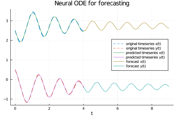
Visualization of original input series, learned series and their future projection
It is clear from the graph that the neural network has learned well the oscillation and damping properties of the two series
and is able to project them into the future.
Note especially the concept of continuous depth typical of NeuralODEs, in fact while in the classical neural networks
the discretization step of the input time series is the same in the forecast, with the NeuralODEs instead the array of the times with which to calculate the prediction can be arbitrarily dense,
with which to calculate the prediction can be arbitrarily dense, just because the solver of differential equations
inside the neural network, by its own nature, works in the continuous and transmits this property to the whole network.
Here the link to the code on GitHub.
Experiment #3: fit a function with MLP and Neural ODEs
Although the Neural ODEs paper does not explicitly mention feature approximation with MLPs
(Multi Layer Perceptron for short) a field of application that could benefit from Neural ODEs,
however it is interesting to see how to build a neural network constituted by a MLP and a layer
to continuous depth implemented through a layer of Neural ODE type.
The experiment has two goals:
-
Show how to define an MLP using
FastChainandFastDensedefined in DiffEqFlux (as opposed to previous experiments whereChainandDensewere used then they were from Flux) without using Neural ODE to approximate a function. - Graft a Neural ODE layer onto the MLP type network and show the necessary changes that need to be made to the code to use this combination of MLP and Neural ODE to approximate the same function.
The application scenario
The application scenario is as follows:
-
A dataset that contains a mapping of real input values (variable $t$, time) to real output values (variable $y$).
The dataset is created synthetically via a generating function $y=y(t)$.
- Fit with a neural network the input $\to$ output mapping represented by the dataset.
The problem to be solved
Let the following generating function of the dataset (which then becomes the function to be fitted) be given:
$$ y(t) = \ln{(1 + t)} - 3 \sqrt {t} \:\:\:\: t \in [0,4] $$
where time $t$ is discretized from $0$ to $4$ with a number of $51$ discrete values;
of course in the real world the dataset is obtained by performing real measurements in the field,
here instead it is generated by a generating function for demonstration purposes..
The problem to be solved, as already mentioned, is to train a neural network to approximate this function by training the neural network
(at first a pure MLP, then a MLP combined with a Neural ODE layer) on the dataset generated via the above generating function.
Solution implementation without Neural ODE
The using statements needed for the entire program are as follows:
using Plots
using Flux
using DiffEqFluxdataset_in and dataset_out:
the first contains the time $t \in [0, 4]$ discretized to have 51 distinct equispaced values,
the second contains the value of the generating function for each discrete value of $t$.The code is:
tbegin = 0.0
tend = 4.0
datasize = 51
dataset_in = range(tbegin, tend, length=datasize)
dataset_out = log.(1 .+ dataset_in) .- 3 * sqrt.(dataset_in)function neural_network(data_dim)
fc = FastChain(FastDense(data_dim, 64, swish),
FastDense(64, 32, swish),
FastDense(32, data_dim))
end
nn = neural_network(1)
theta = initial_params(nn)nn is the MLP neural network and theta is the array of network parameters to be trained.The taxonomy of the neural network is that of a pure MLP (so full connected) structured as follows:
- Number of dimension of input layer: 1
- Number of dimension of outout layer: 1
- Hidden layers: 2 layers, one with 64 neurons and one with 32
- Activation function: swish
The code is:
predict(t, p) = nn(t', p)'

loss(p) = begin
  yhat = predict(dataset_in, p)
  l = Flux.mse(yhat, dataset_out)
end- Optimizator: ADAMW
- Learning rate: $0.01$
- Number of epochs: $1500$
- Loss function: MSE
y_pred
contains the approximation of the generating function:learning_rate=1e-2
opt = ADAMW(learning_rate)
epochs = 1500
function cb_train(theta, loss)
println("Loss: ", loss)
false
end
res_train = DiffEqFlux.sciml_train(
loss, theta, opt,
maxiters = epochs,
cb = cb_train)
y_pred = predict(dataset_in, res_train.minimizer)Note: Given the stochastic nature of the training phase, your specific results may vary. Consider running the training phase a few times.
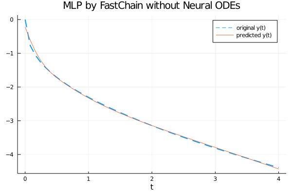
Visualizing the graph of the generating function and the approximation calculated by the MLP neural network
From the graph it is clear that the neural network fits well the generatrix function in the interval $[0, 4]$.
Here the link to the code on GitHub.
Solution implementation with Neural ODE
The using statements needed for the entire program are as follows:
using Plots
using Flux
using DiffEqFlux
using OrdinaryDiffEqOrdinaryDiffEq has been added in order to use NeuralODE.The first part of the program (like the previous program) performs dataset generation which is implemented by two parallel arrays
dataset_in and dataset_out:
the first contains the time $t \in [0, 4]$ discretized to have 51 distinct equispaced values,
the second contains the value of the generating function for each discrete value of $t$.The code is:
tbegin = 0.0
tend = 4.0
datasize = 51
dataset_in = range(tbegin, tend, length=datasize)
dataset_out = log.(1 .+ dataset_in) .- 3 * sqrt.(dataset_in)function neural_ode(data_dim; saveat = dataset_in)
fc = FastChain(FastDense(data_dim, 64, swish),
FastDense(64, 32, swish),
FastDense(32, data_dim))
n_ode = NeuralODE(
fc,
(minimum(dataset_in), maximum(dataset_in)),
Tsit5(),
saveat = saveat,
abstol = 1e-9, reltol = 1e-9)
end
n_ode = neural_ode(1)
theta = n_ode.pn_ode is the Neural ODE neural network and theta is the array of parameters of the Neural ODE network to be trained.The neural network taxonomy is a Neural ODE layer that takes the previous MLP network as an argument.
The prediction function has a variation from the previous case: here in fact the prediction function is not passed the entire input but only the first data, which is intended as a condition for the initial values of a Cauchy problem; the loss function is always the mean square error (MSE for short) between the output dataset and the prediction.
predict(p) = n_ode(dataset_out[1:1], p)'

loss(p) = begin
  yhat = predict(p)
  l = Flux.mse(yhat, dataset_out)
end- Optimizator: ADAMW
- Learning rate: $0.01$
- Number of epochs: $500$
- Loss function: MSE
y_pred
contains the approximation of the generating function:learning_rate=1e-2
opt = ADAMW(learning_rate)
epochs = 500
function cb_train(theta, loss)
println("Loss: ", loss)
false
end
res_train = DiffEqFlux.sciml_train(
loss, theta, opt,
maxiters = epochs,
cb = cb_train)
y_pred = predict(res_train.minimizer)Note: Given the stochastic nature of the training phase, your specific results may vary. Consider running the training phase a few times.
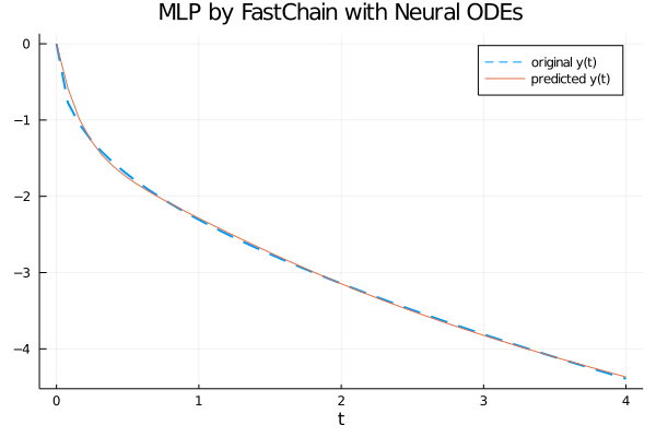
Visualizing the graph of the generating function and the approximation calculated by the MLP neural network with a Neural ODE layer
From the graph it is clear that the neural network with a Neural ODE layer fits well the generatrix function in the interval $[0, 4]$.
Here the link to the code on GitHub.
Citations
@articleDBLP:journals/corr/abs-1806-07366,
  author    = {Tian Qi Chen and
               Yulia Rubanova and
               Jesse Bettencourt and
               David Duvenaud},
  title     = {Neural Ordinary Differential Equations},
  journal   = {CoRR},
  volume    = {abs/1806.07366},
  year      = {2018},
  url       = {http://arxiv.org/abs/1806.07366},
  archivePrefix = {arXiv},
  eprint    = {1806.07366},
  timestamp = {Mon, 22 Jul 2019 14:09:23 +0200},
  biburl    = {https://dblp.org/rec/journals/corr/abs-1806-07366.bib},
  bibsource = {dblp computer science bibliography, https://dblp.org}
@articleDBLP:journals/corr/abs-1902-02376,
  author    = {Christopher Rackauckas and
               Mike Innes and
               Yingbo Ma and
               Jesse Bettencourt and
               Lyndon White and
               Vaibhav Dixit},
  title     = {DiffEqFlux.jl - {A} Julia Library for Neural Differential Equations},
  journal   = {CoRR},
  volume    = {abs/1902.02376},
  year      = {2019},
  url       = {https://arxiv.org/abs/1902.02376},
  archivePrefix = {arXiv},
  eprint    = {1902.02376},
  timestamp = {Tue, 21 May 2019 18:03:36 +0200},
  biburl    = {https://dblp.org/rec/bib/journals/corr/abs-1902-02376},
  bibsource = {dblp computer science bibliography, https://dblp.org}
Download of the complete code
The complete code is available at GitHub.
These materials are distributed under MIT license; feel free to use, share, fork and adapt these materials as you see fit.
Also please feel free to submit pull-requests and bug-reports to this GitHub repository or contact me on my social media channels available on the top right corner of this page.